Multivariable Calculus 16 | Taylor's Theorem

Taylor’s theorem in multivariable calculus generalizes the familiar idea of approximating a smooth function near an expansion point with a polynomial whose coefficients come from derivatives. The practical payoff is that, for a function f: R^n → R (or more generally between Euclidean spaces), values near x̃ can be approximated by a kth-order Taylor polynomial in the displacement h, with a remainder term that quantifies how the approximation error shrinks as h → 0.

The construction starts with the linear approximation. For a small shift from the expansion point x̃ to x̃ + h, differentiability yields a first-order estimate: f(x̃ + h) is approximately f(x̃) plus a linear map applied to h. In multivariable form, that linear map is represented using the Jacobian matrix J_f, so the linear term becomes the matrix-vector product J_f(x̃)·h. The quality of this approximation is measured by an error term Φ(h) that satisfies Φ(h)/||h|| → 0 as ||h|| → 0, ensuring the error is of smaller order than the linear part.

Next comes the quadratic approximation, where the second-order behavior is captured by a polynomial involving second partial derivatives. The quadratic term uses the Hessian matrix H (often denoted with a capital H), and the displacement h enters twice through the bilinear form h^T H h. As with the linear case, a remainder term Ψ(h) accounts for the leftover error, with the requirement that Ψ(h)/||h||^2 → 0 as ||h|| → 0 so the quadratic approximation improves at the expected rate.

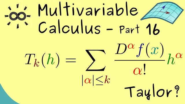
With these pieces in place, the full kth-order Taylor theorem is stated under smoothness assumptions: if f has continuous partial derivatives up to order k+1 (written as f ∈ C^{k+1}(R^n)), then for x̃ and h in R^n, f(x̃ + h) equals the kth-order Taylor polynomial T_k(x̃, h) plus a remainder term R_k. The Taylor polynomial is expressed using multi-index notation. For each multi-index α with |α| ≤ k, the coefficient involves the partial derivative D^α f evaluated at x̃, divided by α!; the corresponding term multiplies by h^α, where h^α denotes the product of the components of h raised to the powers given by α. Summing over all such α produces a polynomial whose highest degree is k.

The remainder term R_k has a “last-order derivatives” structure similar in form to the polynomial itself, but it uses derivatives of order k+1 evaluated at an intermediate point c. That point c lies on the line segment between x̃ and x̃ + h, generalizing the one-dimensional intermediate-point idea. When n = 1, the multivariable statement collapses back to the standard Taylor theorem from real analysis, confirming the consistency of the generalization. The next step is to work through examples to make these formulas concrete.