Multivariable Calculus 18 | Local Extrema
Based on The Bright Side of Mathematics's video on YouTube. If you like this content, support the original creators by watching, liking and subscribing to their content.
A local maximum at x0 requires f(x0) ≥ f(x) for all points x in some ε-neighborhood intersected with the domain.
Briefing
Local extrema in multivariable calculus are defined by comparing function values only within a small neighborhood around a point, not across the entire domain. A function f has a local maximum at x0 if there exists an ε-neighborhood around x0 such that f(x0) is greater than or equal to f(x) for every x in the domain that lies in that neighborhood. The “local” part matters: what happens far away from x0 is irrelevant. For constant functions, this non-strict inequality creates local maxima everywhere, so the notion of an isolated local maximum tightens the idea by requiring a strict inequality—f(x0) must be strictly greater than nearby values except at x0 itself. Local minima mirror this definition with the inequality reversed.
A local extremum means either a local maximum or a local minimum. Once f is assumed continuously differentiable on R^N, a necessary condition emerges: if f has a local extremum at x0, then the gradient must vanish there. In multivariable terms, the gradient ∇f(x0) = 0 vector is the multivariable analogue of “the first derivative is zero” from single-variable calculus. Intuitively, the gradient points in the direction of fastest increase; at a local extremum, there should be no direction that increases the function.
To go beyond necessity and decide whether a critical point is truly a maximum or minimum, the discussion uses a second-order Taylor expansion for C^3 functions. With x0 as a critical point (∇f(x0)=0), the quadratic approximation near x0 becomes f(x0+h) ≈ f(x0) + (1/2) h^T H_f(x0) h, where H_f(x0) is the Hessian matrix of second partial derivatives. The Hessian then determines the local shape: - If H_f(x0) is positive definite—meaning h^T H_f(x0) h is strictly positive for every nonzero h—then f has an isolated local minimum at x0. - If H_f(x0) is negative definite—meaning h^T H_f(x0) h is strictly negative for every nonzero h—then f has an isolated local maximum at x0. - If the Hessian is indefinite, so there exist directions h1 and h2 with opposite signs (one giving positive and the other negative quadratic behavior), then x0 is not a local extremum. Instead, the point behaves like a saddle point: the function rises in some directions and falls in others.
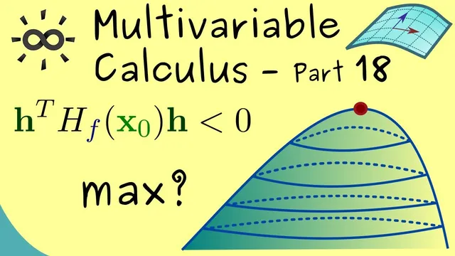
The transcript also notes one-way implications when starting from the existence of an extremum. If f has a local maximum at x0, the Hessian must be negative semi-definite (h^T H_f(x0) h ≤ 0 for all h), allowing zero values in some directions; similarly, a local minimum forces the Hessian to be positive semi-definite. Because semi-definiteness can occur even when the extremum is not isolated, the converse statements (definiteness/semi-definiteness implying an extremum) do not always hold without the strict definiteness conditions. The practical takeaway is that the Hessian’s definiteness classifies critical points into isolated minima, isolated maxima, saddle points, or cases where the test is inconclusive—setting up the next step: working through examples.
Cornell Notes
The core goal is to classify local maxima and minima of a multivariable function f: R^N → R using the gradient and the Hessian. A local maximum at x0 occurs when f(x0) is at least as large as nearby values within some ε-neighborhood; an isolated local maximum requires strict inequality for all nearby points except x0. For continuously differentiable functions, any local extremum forces the gradient to vanish: ∇f(x0)=0. For C^3 functions, the second-order Taylor approximation shows that the Hessian H_f(x0) determines the outcome: positive definite Hessian ⇒ isolated local minimum; negative definite Hessian ⇒ isolated local maximum; indefinite Hessian ⇒ saddle point (no local extremum). If only a local maximum/minimum is assumed, the Hessian must be negative/positive semi-definite, but semi-definiteness alone may not guarantee an isolated extremum.
How do definitions of local maximum and isolated local maximum differ, and why does that matter for constant functions?
Why must the gradient vanish at a local extremum for C^1 functions?
What does the Hessian tell you once ∇f(x0)=0, and how does the quadratic approximation enter?
How do positive definite, negative definite, and indefinite Hessians correspond to minima, maxima, and saddle points?
Why do semi-definite Hessians give only one-way conclusions?
Review Questions
- Suppose ∇f(x0)=0 and the Hessian H_f(x0) is indefinite. What can be concluded about local extrema at x0?
- State the necessary condition for a local extremum in terms of the gradient for continuously differentiable functions.
- Explain the difference between positive definite and positive semi-definite Hessians and how each affects the classification of x0.
Key Points
- 1
A local maximum at x0 requires f(x0) ≥ f(x) for all points x in some ε-neighborhood intersected with the domain.
- 2
An isolated local maximum strengthens this to f(x0) > f(x) for all nearby x ≠ x0, preventing constant functions from creating infinitely many local maxima.
- 3
For continuously differentiable functions, any local extremum at x0 forces the gradient to vanish: ∇f(x0)=0.
- 4
For C^3 functions, the second-order Taylor approximation near a critical point uses the Hessian matrix to determine local behavior.
- 5
Positive definite Hessian implies an isolated local minimum; negative definite Hessian implies an isolated local maximum.
- 6
Indefinite Hessian implies a saddle point, so no local extremum exists at x0.
- 7
If a local maximum/minimum is known to exist, the Hessian must be negative/positive semi-definite, but semi-definiteness alone is not sufficient for an isolated extremum.