Multivariable Calculus 28 | Extreme Values With Constraints

Local maxima and minima of multivariable functions usually come from where the gradient vanishes. That rule breaks down once the search is restricted to a constraint set—like a curve on a surface—because the function can still have nonzero gradient everywhere along the allowed points. The key fix is the method of Lagrange multipliers: at a constrained local extremum, the gradient of the objective function must align with the gradient of the constraint.

The discussion starts with a standard setup: for a C1 function f on an open subset of R2, local extrema can only occur at points where ∇f = 0. Geometrically, contour lines of f show where f is constant, and ∇f is perpendicular to those contours. If ∇f is not zero, moving in the gradient direction increases f, so an interior local extremum cannot happen.

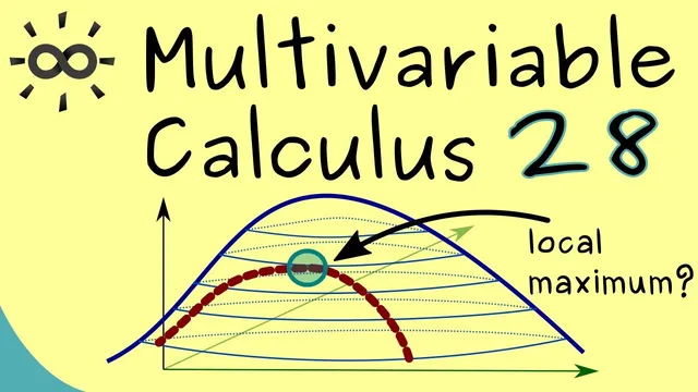
Next comes the constrained version. Suppose the constraint is given by a C1 function G(x, y) = 0, which defines a curve in R2. Instead of optimizing f over all of R2, the goal is to optimize the restriction of f to the set G = {x ∈ R2 : G(x) = 0}. On this curve, the earlier “∇f = 0” condition becomes useless: the gradient of f can be nonzero at every point on the curve, even though the constrained maximum still exists. The geometric reason is that allowed moves are only along the constraint curve; the gradient direction may point off the curve, so it no longer guarantees an increase within the feasible set.

At a constrained local maximum, the contour of f must be tangent to the constraint curve. In gradient language, this means the direction perpendicular to the f-contours (∇f) must match the direction perpendicular to the constraint curve (∇G). Since ∇G is perpendicular to the contour line G = 0, the constrained extremum occurs precisely when ∇f and ∇G lie in the same one-dimensional subspace—equivalently, when ∇f is parallel to ∇G.

Formally, for a point x̃ on the constraint (so G(x̃) = 0), a necessary condition for f to have a local extremum subject to the constraint is that there exists a real number λ such that ∇f(x̃) = λ ∇G(x̃).

A second requirement is included to keep the constraint well-behaved: ∇G(x̃) must not be the zero vector, so the constraint curve has a meaningful tangent direction (it spans a one-dimensional subspace). The resulting implication is necessary but not sufficient: solving for points x̃ and multipliers λ that satisfy the equation identifies the only candidates for constrained extrema, but additional checks are still needed to confirm which candidates are actual maxima or minima.

The takeaway is practical and geometric at once: constrained extrema happen where the objective’s gradient lines up with the constraint’s gradient, with the scalar λ measuring how strongly the constraint “scales” that alignment.