Multivariable Calculus 4 | Partial Derivatives

Partial derivatives turn multivariable differentiation into a sequence of ordinary one-variable derivatives by freezing all but one coordinate. That shift matters because it gives a precise way to measure how a function changes when only one input direction varies—an idea that underpins gradients, tangent planes, and optimization in higher dimensions.

The discussion starts by connecting continuity and differentiability to “all possible approximations.” For functions on the plane, continuity at a point requires that values along any converging sequence approach the function’s value. Derivatives inherit the same spirit: instead of only looking along coordinate axes, multivariable differentiation must account for how changes behave when inputs approach a point in specific ways. The simplest derivatives that come directly from the one-dimensional case are the partial derivatives.

To define them, the transcript emphasizes notation for functions of vectors. A function value can be written as f(x) where x is a vector (x1, x2, …, xn), or equivalently by explicitly listing components as f(x1, x2, …, xn). For partial derivatives, the key move is to fix all coordinates except one. For example, to study differentiability with respect to x1 at a point x~ = (x~1, x~2, …, x~n), all other variables are held constant at their values in x~. What remains is an ordinary single-variable function of x1: x1 ↦ f(x1, x~2, …, x~n). If the usual one-dimensional derivative of this function exists, then f is partially differentiable with respect to x1 at x~.

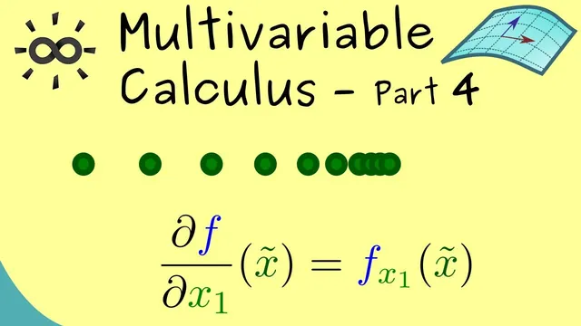
Formally, the partial derivative with respect to x1 is defined by the limit of the difference quotient where only x1 changes: [f(x~1 + h, x~2, …, x~n) − f(x~1, x~2, …, x~n)] / h, with h → 0. The transcript notes that differentiability is pointwise, so the point x~ must appear in the notation. It also surveys common ways partial derivatives are written—using symbols like ∂/∂x1, sometimes with subscripts or alternative d-notations—while stressing that the evaluation point should not be forgotten.

The same construction applies to x2, x3, and any xi: only the chosen coordinate gets the +h perturbation, while the rest stay fixed. The examples make the mechanics concrete using a function from R^3 to R: f(x1, x2, x3) = x1^2 · x2 · sin(x3). The partial derivative with respect to x1 treats x2 and sin(x3) as constants, yielding 2x1 · x2 · sin(x3) evaluated at the chosen point. With respect to x2, the derivative of the linear factor x2 gives x1^2 · sin(x3). With respect to x3, the derivative of sin(x3) becomes cos(x3), producing x1^2 · x2 · cos(x3).

A final takeaway addresses constants: if x3 is added to the original function, then in the partial derivative with respect to x3 that added x3 contributes a derivative of 1, while partial derivatives with respect to x1 or x2 remain unchanged because x3 acts like a constant when those other variables vary. The groundwork is then set for later types of derivatives beyond partial derivatives.