Newton’s Fractal is beautiful

TL;DR

Newton’s method approximates solutions to f(x)=0 by iterating tangent-line updates: start with a guess, move using the tangent intersection rule, and repeat.

Briefing Cornell Notes

Briefing

Newton’s fractal turns a classic calculus algorithm—Newton’s method for solving equations—into a mesmerizing map of the complex plane. The core idea is simple: pick an initial guess, apply Newton’s update rule to move the guess closer to a root, and repeat. When this process is run for every possible starting point (at pixel-level resolution), the plane doesn’t just fill with random outcomes; it organizes into sharp, repeating color regions that reveal which root each starting point converges to. That structure is what produces Newton’s fractal, and it comes as an infinite family depending on the polynomial being solved.

Newton’s method begins with an equation rewritten as f(x)=0. In the real-number setting, the geometric meaning is intuitive: a solution is where the graph of f crosses the x-axis. Starting from a guess x0, the method draws the tangent line to f at x0, finds where that tangent intersects the x-axis, and uses that intersection as the next approximation. Repeating this “tangent-intersect-update” often drives the guesses toward an actual root quickly, and the step size can be derived from calculus.

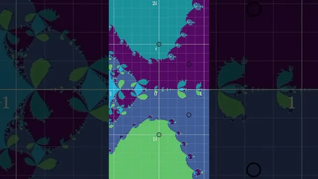
The fractal magic appears when the same update rule is applied to complex numbers. The tangent-line picture no longer translates directly into a simple x-axis crossing story, but the formula still defines how to iterate guesses in the complex plane. For a degree-5 polynomial, there are five distinct complex roots. If many starting points are iterated, most of them eventually “zero in” on one of those roots. Coloring each starting point by the root it converges to—then rewinding to see where each colored point began—creates a structured pattern. At high resolution, treating each pixel as a separate initial guess, the resulting root-attraction map becomes the familiar Newton’s fractal image: an infinitely detailed, boundary-rich mosaic where neighboring starting points can land in different roots.

The transcript also hints at why this matters beyond aesthetics. The fractal patterns reflect how Newton’s method behaves in practice: convergence speed and success depend sensitively on the starting point, especially near the complicated boundaries between basins of attraction. Those same ideas connect to other famous complex dynamics objects, including the Mandelbrot set. In short, Newton’s method doesn’t just approximate solutions—it partitions the complex plane into basins whose borders encode the algorithm’s stability, and the resulting partition is fractal, beautiful, and deeply informative.

Cornell Notes

Newton’s fractal is built by running Newton’s method on complex numbers for an equation f(z)=0. Each initial guess z0 is iteratively updated using the Newton step derived from calculus, and the iteration converges to one of the polynomial’s roots (when it converges). For a degree-5 polynomial, there are five roots, so the complex plane can be colored by which root each starting point approaches. Rendering this coloring at pixel-level resolution produces an intricate, infinitely detailed boundary structure between “basins of attraction.” These fractals matter because they show how sensitive Newton’s method can be to the starting guess, especially near the borders, and they connect to broader themes in complex dynamics such as the Mandelbrot set.

How does Newton’s method move a guess toward a root in the real-number setting?

Rewrite the equation as f(x)=0. Start with an initial guess x0, draw the tangent line to y=f(x) at x0, and compute where that tangent line intersects the x-axis. Use that intersection as the next approximation x1. Repeat the process; with the calculus-derived step-size rule, the iterates often converge quickly to a solution.

Why can Newton’s method be applied to complex numbers even though the geometric picture changes?

The transcript notes that while the real-number visualization (tangent lines and x-axis crossings) doesn’t carry over directly to complex inputs, the Newton update formula still defines a valid iteration rule for complex guesses. So the method remains a rule for adjusting z to get closer to a complex root, even without the same simple geometric interpretation.

What does it mean to “color” Newton’s fractal, and what determines each color?

For a polynomial of degree 5, there are five distinct complex solutions (roots). After iterating Newton’s method from many starting points, each starting point converges to one of those roots (or fails to converge). The coloring assigns each starting point a color based on which root it ends up closest to, producing regions corresponding to different basins of attraction.

How does the fractal image emerge when every pixel is treated as an initial guess?

At very fine resolution, each pixel location in the complex plane is treated as a separate initial guess. Newton’s method is iterated from each pixel, and the pixel is colored by the root it converges to. The final rendered image is the Newton’s fractal: a structured pattern whose boundaries are extremely intricate, reflecting how convergence outcomes change under tiny changes in the starting point.

What practical lesson about Newton’s method is suggested by the fractal boundaries?

The transcript points to sensitivity: near the complicated borders between basins of attraction, tiny differences in the initial guess can send iterations toward different roots. That means success and behavior of Newton’s method depend strongly on where you start, not just on the equation itself.

Review Questions

For f(z)=0 with a degree-5 polynomial, how many distinct roots should Newton’s method converge to (in the typical case), and how does that number affect the coloring scheme?
Why does treating each pixel as a different initial guess produce a structured image rather than a random scatter of outcomes?
What does the existence of intricate basin boundaries imply about the stability of Newton’s method with respect to the starting guess?

Key Points

1
Newton’s method approximates solutions to f(x)=0 by iterating tangent-line updates: start with a guess, move using the tangent intersection rule, and repeat.
2
The calculus-derived Newton update rule still works when the input and output are complex numbers, even though the real-number geometric picture no longer applies.
3
For a degree-5 polynomial, there are five complex roots, so the complex plane can be partitioned into five basins of attraction.
4
Running Newton’s method from many initial guesses and coloring each guess by the root it converges to produces Newton’s fractal.
5
At high resolution, treating each pixel as an initial guess yields an infinitely detailed boundary structure between regions that converge to different roots.
6
The fractal structure reflects how sensitive Newton’s method can be near basin boundaries, affecting convergence behavior in practice.
7
Newton’s fractals connect to broader complex dynamics themes, including the Mandelbrot set.

Highlights

Newton’s method can be turned into a visual “root-attraction map” by iterating from every starting point in the complex plane.

For a degree-5 polynomial, the complex plane splits into five colored regions—each corresponding to which of the five roots the iteration approaches.

Even without the real-number tangent-and-x-axis geometry, the Newton update formula still drives complex iterations toward roots.

The most striking feature is the infinitely detailed, boundary-rich pattern where tiny changes in the starting guess can change the final root.

Topics

Newton’s Method
Complex Roots
Fractals
Basins of Attraction
Complex Dynamics