Why is choosing $\tilde\alpha(t)=1$ valid for $\dot x=x$ with $x(0)=1$?

Picard iteration only requires the starting guess to satisfy the initial value equation at $t=0$. The constant function $\tilde\alpha(t)=1$ meets $\tilde\alpha(0)=1$, so it can serve as the initial guess even if it is not the true solution.

Ordinary Differential Equations 13

Q: How is Picard iteration constructed from the fixed-point map $F$?

One starts with any function $\tilde\alpha$ satisfying the initial condition. Then repeatedly apply the integral operator $F$: $\tilde\alpha,\; F(\tilde\alpha),\; F^2(\tilde\alpha),\ldots$. Because $F$ is defined using one integral, applying it $n$ times corresponds to $n$ integrations in a row.

Q: How do the iterates generate the exponential series for $\dot x=x$?

The first iterate gives $1+t$. The second iterate integrates the linear function inside the integral, producing $1+t+\tfrac{1}{2}t^2$. Repeating the process adds higher powers of $t$ with factorial denominators; the $n$-th step contributes a term $\tfrac{1}{n!}t^n$. The pointwise limit becomes $\sum_{k=0}^\infty \tfrac{t^k}{k!}=e^t$.

TL;DR

Picard–Lindelöf theory links existence and uniqueness of solutions to a fixed-point construction that can be used for approximation.

Briefing Cornell Notes

Briefing

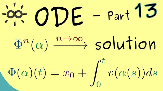
Picard–Lindelöf theory doesn’t just guarantee that an initial value problem has a unique solution—it also provides a practical way to approximate that solution via Picard iteration. Under a local Lipschitz condition, the initial value problem has a unique solution, and the proof can be turned into an iterative scheme: start from any initial guess function $\tilde{α}$ , apply a fixed-point map $F$ repeatedly, and take the limit as the number of iterations $n \to \infty$ . Because each application of $F$ involves one integral, composing $F$ $n$ times produces $n$ nested integrations. This is the mechanism behind Picard iteration—less “magic” and more a direct consequence of the fixed-point argument.

To make the iteration concrete, the transcript works through the differential equation $\overset{x}{˙} = x$ with initial condition $x (0) = 1$ . The corresponding vector field is the identity map, so the integral form of the problem becomes $x (t) = 1 + \int_{0}^{t} x (s) d s$ . Picard iteration begins with a function $\tilde{α}$ that only needs to satisfy the initial condition at $t = 0$ . Choosing the simplest option, the constant function $\tilde{α} (t) = 1$ , the first iterate is computed by plugging into the integral: $F (\tilde{α}) (t) = 1 + \int_{0}^{t} 1 d s = 1 + t$ . The second iterate replaces the integrand with the new function, giving $F^{2} (\tilde{α}) (t) = 1 + \int_{0}^{t} (1 + s) d s = 1 + t + \frac{1}{2} t^{2}$ .

Continuing this pattern, each iteration adds the next term in a power series. The transcript highlights that after repeating the integration process, the $n$ -th step produces a polynomial whose highest-degree term scales like $\frac{1}{n !} t^{n}$ . By induction (suggested as a straightforward verification), the general form emerges: the iterates build the truncated Taylor series of the exponential function. Taking the limit pointwise as $n \to \infty$ yields the infinite series $\sum_{k = 0}^{\infty} \frac{t ^{k}}{k !}$ , which is exactly $e^{t}$ . Thus the iteration converges to $x (t) = e^{t}$ , matching the known closed-form solution.

A key theoretical payoff is that fixed-point machinery upgrades convergence. The iteration converges by the Banach fixed-point theorem, which implies a unique uniform limit. Since uniform convergence is stronger than pointwise convergence, the limit obtained from the pointwise series must be the same uniform limit—so the example doesn’t need separate work to justify uniform convergence. The result is a clean demonstration: Picard iteration turns the existence/uniqueness theorem into an explicit computational method, and for $\overset{x}{˙} = x$ it reproduces the exponential function term-by-term. The next step in the series is to connect these results to the geometry of solution curves and their “orbits.”

Cornell Notes

Picard–Lindelöf theory guarantees a unique solution to an initial value problem when the right-hand side satisfies a local Lipschitz condition. The proof also yields Picard iteration: define an integral operator $F$ and repeatedly apply it to an initial guess $\tilde{α}$ that only needs to satisfy the initial condition. Each application of $F$ adds one more integration, so $F^{n}$ corresponds to $n$ nested integrals. For $\overset{x}{˙} = x$ , starting from $\tilde{α} (t) = 1$ produces iterates that build the series $1 + t + \frac{1}{2} t^{2} + \dots + \frac{1}{n !} t^{n}$ , which converges to $e^{t}$ . Banach fixed-point theory ensures the convergence is uniform, so the pointwise limit from the series is the actual solution.

What role does the local Lipschitz condition play in Picard–Lindelöf theory?

It’s the condition that makes the fixed-point map behave well enough to guarantee a unique solution. With local Lipschitz continuity in place, the initial value problem has a unique solution, and the fixed-point framework can be used to approximate it via iteration.

How is Picard iteration constructed from the fixed-point map $F$ ?

One starts with any function

\tilde{α}

satisfying the initial condition. Then repeatedly apply the integral operator

F

\tilde{α}, F (\tilde{α}), F^{2} (\tilde{α}), \dots

. Because

F

is defined using one integral, applying it

n

times corresponds to

n

integrations in a row.

Why is choosing $\tilde{α} (t) = 1$ valid for $\overset{x}{˙} = x$ with $x (0) = 1$ ?

Picard iteration only requires the starting guess to satisfy the initial value equation at

t = 0

. The constant function

\tilde{α} (t) = 1

meets

\tilde{α} (0) = 1

, so it can serve as the initial guess even if it is not the true solution.

How do the iterates generate the exponential series for $\overset{x}{˙} = x$ ?

The first iterate gives

1 + t

. The second iterate integrates the linear function inside the integral, producing

1 + t + \frac{1}{2} t^{2}

. Repeating the process adds higher powers of

t

with factorial denominators; the

n

-th step contributes a term

\frac{1}{n !} t^{n}

. The pointwise limit becomes

\sum_{k = 0}^{\infty} \frac{t ^{k}}{k !} = e^{t}

What does Banach fixed-point theory add beyond pointwise convergence in this example?

It ensures the iteration converges to a unique fixed point with uniform convergence. Since uniform convergence implies pointwise convergence, the pointwise series limit already identifies the uniform limit, so the exponential obtained from the series is guaranteed to be the actual solution.

Review Questions

For $\overset{x}{˙} = x$ with $x (0) = 1$ , compute $F (\tilde{α}) (t)$ and $F^{2} (\tilde{α}) (t)$ starting from $\tilde{α} (t) = 1$ .
Explain why $F^{n}$ corresponds to $n$ nested integrations and how that leads to a power series.
What is the relationship between the pointwise limit of Picard iterates and the uniform limit guaranteed by the Banach fixed-point theorem?

Key Points

1
Picard–Lindelöf theory links existence and uniqueness of solutions to a fixed-point construction that can be used for approximation.
2
Picard iteration applies an integral operator $F$ repeatedly to an initial guess $\tilde{α}$ satisfying only the initial condition.
3
Each iteration adds one more integration, so $F^{n}$ corresponds to $n$ integrations in sequence.
4
For $\overset{x}{˙} = x$ with $x (0) = 1$ , starting from $\tilde{α} (t) = 1$ generates $1 + t + \frac{1}{2} t^{2} + \dots$ , matching the exponential series.
5
The $n$ -th iterate produces a term with coefficient $\frac{1}{n !}$ in front of $t^{n}$ , which can be justified by induction.
6
The Banach fixed-point theorem guarantees uniform convergence to the unique solution, so the pointwise series limit identifies the true solution.
7
The example demonstrates how the abstract fixed-point proof becomes an explicit computational method for solving ODEs.

Highlights

Picard iteration turns the fixed-point proof into an algorithm: apply the integral operator F over and over and take the limit.

For x˙=x, the iterates build the exponential series term-by-term, converging to et.

Uniform convergence is guaranteed by Banach fixed-point theory, so the series limit obtained pointwise is automatically the correct solution.

Topics

Mentioned

ODE
P
$F$

Ordinary Differential Equations 13 | Picard Iteration

Briefing

Cornell Notes

What role does the local Lipschitz condition play in Picard–Lindelöf theory?

How is Picard iteration constructed from the fixed-point map $F$ ?

Why is choosing $\tilde{α} (t) = 1$ valid for $\overset{x}{˙} = x$ with $x (0) = 1$ ?

How do the iterates generate the exponential series for $\overset{x}{˙} = x$ ?

What does Banach fixed-point theory add beyond pointwise convergence in this example?

Review Questions

Key Points

Highlights

Topics

Mentioned

Get summaries like this for any content

Briefing

Cornell Notes

What role does the local Lipschitz condition play in Picard–Lindelöf theory?

How is Picard iteration constructed from the fixed-point map F?

Why is choosing α~(t)=1 valid for x˙=x with x(0)=1?

How do the iterates generate the exponential series for x˙=x?

What does Banach fixed-point theory add beyond pointwise convergence in this example?

Review Questions

Key Points

Highlights

Topics

Mentioned

Get summaries like this for any content

How is Picard iteration constructed from the fixed-point map $F$ ?

Why is choosing $\tilde{α} (t) = 1$ valid for $\overset{x}{˙} = x$ with $x (0) = 1$ ?

How do the iterates generate the exponential series for $\overset{x}{˙} = x$ ?