Ordinary Differential Equations 17 | Picard–Lindelöf Theorem (General and Special Version)
Based on The Bright Side of Mathematics's video on YouTube. If you like this content, support the original creators by watching, liking and subscribing to their content.
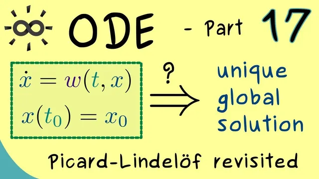
For x'(t)=W(t,x(t)), local existence and uniqueness follow from Lipschitz continuity in x (the second argument), not necessarily in t.
Briefing
Picard–Lindelöf gets a nonautonomous upgrade: for initial value problems where the dynamics depend on time as well as state, a locally Lipschitz condition in the state variable guarantees both existence and uniqueness of solutions. The key shift is replacing the autonomous vector field V(x) with a two-input map W(t, x), then requiring Lipschitz control only in the second argument. Concretely, around any initial point (t0, x0), one can choose a neighborhood shaped like a generalized rectangle (a time interval times an open set in state space) and demand that for all points in that rectangle, the inequality ||W(t, x) − W(t, y)|| ≤ L_K ||x − y|| holds with the same Lipschitz constant for each fixed time slice. Under that local condition, the initial value problem has a unique solution defined on some time interval (t0 − ε, t0 + ε), and the solution can be extended to a maximal one.
The proof strategy stays essentially the same as in the autonomous case: it still leans on the Banach fixed point theorem. The fixed-point map is adjusted by swapping the autonomous vector field V for the nonautonomous W, turning the candidate solution α into a function satisfying an integral equation. Instead of using x0 + ∫ V(s, α(s)) ds, the construction uses x0 + ∫_{t0}^{T} W(s, α(s)) ds, so the Lipschitz property in x is what drives the contraction argument. That means the existence-and-uniqueness machinery doesn’t require new tools—just the right Lipschitz hypothesis and the same integral formulation.
Beyond the general nonautonomous version, a special “global solution” form is presented for applications. Here W is continuous on the full domain R × R^N and satisfies a global Lipschitz condition in x: a single Lipschitz constant works for every pair of states, for all x, y in R^N. Time is handled by restricting attention to any finite window [−T, T], with the Lipschitz constant allowed to depend on that window (so it’s uniform in space but not necessarily across all time scales at once). With these stronger assumptions, the theorem yields a unique solution defined for all t ∈ R, not merely on a short interval.
The global proof again uses Banach’s theorem, but it faces a familiar obstacle: the fixed-point map is only a contraction on small time intervals under the standard sup norm. The workaround is to modify the metric on the function space using an exponential weighting factor involving the Lipschitz constant L_T. This reweights points far from the origin in time so that the integral operator becomes a contraction even as the time window grows. After verifying the modified metric remains complete and that the contraction constant can be bounded uniformly, the fixed point produces a unique solution on [−T, T]. Since the construction works for arbitrary T, the solution extends to the entire real line.
Taken together, the result provides a practical roadmap: local Lipschitz control in the state variable gives local uniqueness and existence for time-dependent systems, while global Lipschitz control (with the right uniformity) upgrades that to global-in-time solutions—exactly the kind of guarantee needed before moving on to linear ODEs and their stability properties.
Cornell Notes
For nonautonomous initial value problems of the form x'(t)=W(t,x(t)), Picard–Lindelöf still delivers existence and uniqueness as long as W is Lipschitz in the state variable x. Around any initial point (t0,x0), one can choose a local rectangle in time and state space and require ||W(t,x)−W(t,y)|| ≤ L_K||x−y|| for all points in that rectangle (with L_K depending on the chosen rectangle). Under this local Lipschitz condition, the integral fixed-point map x0+∫_{t0}^{T}W(s,α(s))ds has a unique fixed point, giving a unique solution on some interval and extendable to a maximal solution. A special global version assumes W is continuous on R×R^N and satisfies a global Lipschitz condition in x, enabling a unique solution for all t∈R using an exponentially weighted metric.
How does the Lipschitz requirement change when moving from autonomous systems x'=V(x) to nonautonomous systems x'=W(t,x)?
Why is the “generalized rectangle” (time interval × state neighborhood) used in the nonautonomous theorem?
What fixed-point map replaces the autonomous integral equation in the nonautonomous proof?
Why does the global version need a modified metric instead of the usual sup norm?
What does the global Lipschitz condition buy in terms of the solution’s time domain?
Review Questions
- In the nonautonomous Picard–Lindelöf theorem, what exactly is compared by the Lipschitz inequality—x values at the same time t, or different times?
- What role does the integral equation x0+∫ W(s,α(s)) ds play in the Banach fixed point argument?
- In the global version, how does the exponential weighting in the metric help prevent the contraction constant from worsening as the time interval grows?
Key Points
- 1
For x'(t)=W(t,x(t)), local existence and uniqueness follow from Lipschitz continuity in x (the second argument), not necessarily in t.
- 2
Around any initial point (t0,x0), one can restrict to a local rectangle (time interval × state neighborhood) where a Lipschitz constant L_K works uniformly for all points in that region.
- 3
The proof still uses Banach’s fixed point theorem, with a fixed-point map defined by x0+∫_{t0}^{T}W(s,α(s))ds.
- 4
Under the local Lipschitz condition, the initial value problem has a unique solution on some interval and can be extended to a maximal solution.
- 5
A special global version assumes continuity of W on R×R^N and a global Lipschitz condition in x, yielding a unique solution defined for all t∈R.
- 6
To make the fixed-point map a contraction on large time intervals, the global proof uses an exponentially weighted metric rather than the plain sup norm.