Ordinary Differential Equations 23 | Example for Matrix Exponential

TL;DR

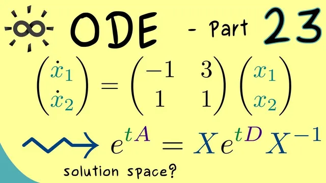
Rewrite the 2×2 system as ẋ = A x, where the solution set is generated by e^{tA}.

Briefing Cornell Notes

Briefing

A 2×2 homogeneous, autonomous linear system can be solved cleanly by converting it into a matrix exponential—then making that exponential computable through diagonalization. The method hinges on rewriting the system as ẋ = A x, where the entire solution set is spanned by the columns of e^{tA}. For the specific system ẋ1 = -x1 + 3x2, ẋ2 = x1 + x2, the coefficient matrix is A = [[-1, 3],[1, 1]]. Solving the system therefore reduces to computing e^{tA}.

The key computational shortcut comes from diagonalizable matrices. If A can be written as A = X D X^{-1}, with D diagonal, then powers become easy: A^k = X D^k X^{-1}. Since the matrix exponential is defined by the power series e^{tA} = Σ_{k=0}^∞ (tA)^k/k!, the same diagonalization trick carries through, yielding e^{tA} = X e^{tD} X^{-1}. That turns an infinite series of matrix powers into a finite sequence of matrix multiplications around a diagonal exponential.

For this example, diagonalization starts with the characteristic polynomial det(A − λI). Computing det([[-1−λ, 3],[1, 1−λ]]) gives λ^2 − 4, so the eigenvalues are λ = −2 and λ = 2. The diagonal matrix D places these values on the diagonal (in the chosen order): D = diag(−2, 2). Next come eigenvectors, found by solving (A − λI)v = 0 for each eigenvalue.

For λ = −2, the matrix A − (−2)I = A + 2I becomes [[1, 3],[1, 3]], whose kernel is one-dimensional and can be spanned by v1 = [−3, 1]^T. For λ = 2, A − 2I = [[-3, 3],[1, -1]] has kernel spanned by v2 = [1, 1]^T. Using these eigenvectors as columns forms the invertible matrix X = [[-3, 1],[1, 1]], with inverse X^{-1} = (1/4) [[-1, 1],[1, 3]].

With D in hand, e^{tD} is immediate because D is diagonal: e^{tD} = diag(e^{-2t}, e^{2t}). Multiplying X e^{tD} X^{-1} produces an explicit closed form for e^{tA}. The resulting matrix entries combine exponentials e^{-2t} and e^{2t} with fixed coefficients; for instance, the (1,1) entry is (1/4)(3e^{-2t} + e^{2t}), and the other entries follow similarly.

Finally, any initial value problem x(0) = x0 is solved by x(t) = e^{tA} x0. Taking x0 = [0, 4]^T selects the second column of e^{tA}, giving a solution whose components are explicit linear combinations of e^{-2t} and e^{2t}. The procedure depends on diagonalizability; when A is not diagonalizable, the appropriate replacement is Jordan normal form, which is flagged as the next step for future treatment.

Cornell Notes

The system ẋ = A x is solved by computing the matrix exponential e^{tA}, because its columns span all solutions. When A is diagonalizable, the exponential becomes practical: if A = X D X^{-1} with D diagonal, then e^{tA} = X e^{tD} X^{-1}. For the example A = [[-1, 3],[1, 1]], the characteristic polynomial det(A − λI) = λ^2 − 4 yields eigenvalues −2 and 2, so D = diag(−2, 2). Eigenvectors give X = [[-3, 1],[1, 1]] and X^{-1} = (1/4)[[-1, 1],[1, 3]]. Then e^{tD} = diag(e^{-2t}, e^{2t}), and multiplying produces an explicit e^{tA}; initial conditions follow from x(t) = e^{tA}x0.

Why does solving ẋ = A x reduce to computing e^{tA}?

For a homogeneous autonomous linear system, the solution set is generated by the matrix exponential. Writing the system as ẋ = A x, the general solution can be expressed using e^{tA}; specifically, the columns of e^{tA} span all solutions. With an initial condition x(0)=x0, the unique solution is x(t)=e^{tA}x0.

How are eigenvalues and eigenvectors used to compute e^{tA} for diagonalizable matrices?

Diagonalization provides A = X D X^{-1}. Eigenvalues become the diagonal entries of D, and eigenvectors form the columns of X. Because A^k = X D^k X^{-1}, the power-series definition of the exponential turns into e^{tA} = X e^{tD} X^{-1}, where e^{tD} is just the exponential applied to each diagonal entry.

What are the eigenvalues for the example matrix A = [[-1, 3],[1, 1]] and how are they found?

Compute the characteristic polynomial det(A − λI). Here det([[-1−λ, 3],[1, 1−λ]]) simplifies to λ^2 − 4. Setting it to zero gives λ = −2 and λ = 2, which become the diagonal entries of D.

How are the eigenvectors chosen for λ = −2 and λ = 2?

For λ = −2, solve (A + 2I)v = 0, which yields a one-dimensional kernel spanned by v1 = [−3, 1]^T. For λ = 2, solve (A − 2I)v = 0, whose kernel is spanned by v2 = [1, 1]^T. Placing these eigenvectors as columns forms X.

How does an initial value x(0) = [0, 4]^T determine x(t)?

Use x(t)=e^{tA}x0. Multiplying by [0, 4]^T selects the second column of e^{tA} and scales it by 4, so each component of x(t) becomes an explicit combination of e^{-2t} and e^{2t} with fixed coefficients.

Review Questions

Given ẋ = A x, what role do the columns of e^{tA} play in describing the solution set?
If A = X D X^{-1} with D diagonal, write the formula for e^{tA} in terms of X, D, and t.
For A = [[-1, 3],[1, 1]], what characteristic polynomial leads to the eigenvalues, and what are those eigenvalues?

Key Points

1
Rewrite the 2×2 system as ẋ = A x, where the solution set is generated by e^{tA}.
2
Use the definition e^{tA} = Σ_{k=0}^∞ (tA)^k/k! to connect the exponential to matrix powers.
3
If A is diagonalizable (A = X D X^{-1}), then A^k = X D^k X^{-1}, making e^{tA} computable as X e^{tD} X^{-1}.
4
Find eigenvalues from det(A − λI)=0; place them on the diagonal of D.
5
Find eigenvectors from (A − λI)v=0; use them as columns of X to build the diagonalization.
6
Compute e^{tD} by exponentiating each diagonal entry, producing diag(e^{λ1 t}, e^{λ2 t}).
7
Solve initial value problems via x(t)=e^{tA}x0; when A is not diagonalizable, switch to Jordan normal form.

Highlights

Diagonalization turns an infinite matrix power series into a simple diagonal exponential: e^{tA} = X e^{tD} X^{-1}.

For A = [[-1, 3],[1, 1]], the characteristic polynomial is λ^2 − 4, giving eigenvalues −2 and 2.

Eigenvectors for −2 and 2 can be chosen as [−3, 1]^T and [1, 1]^T, forming X and enabling an explicit e^{tA}.

With x(0) = [0, 4]^T, the solution x(t) is obtained by taking the second column of e^{tA} and scaling by 4.