Ordinary Differential Equations 24 | Characteristic Polynomial

For linear, homogeneous, autonomous differential equations of order n, the path to the general solution runs through the characteristic polynomial—because it determines the eigenvalues that control the matrix exponential. Start with the standard first-order system form ẋ = A x, where A is an n×n matrix. When the eigenvalues of A are known, the solution set is spanned by columns of e^{tA}, and in the best case (n distinct real eigenvalues) the matrix exponential becomes straightforward to compute via diagonalization. This matters because it turns a higher-order differential equation problem into an eigenvalue problem with a clean algebraic entry point.

The same eigenvalue logic carries over to an nth-order linear homogeneous autonomous ODE: x^{(n)} + a_{n-1}x^{(n-1)} + … + a_1 ẋ + a_0 x = 0. Converting it to a first-order system uses the usual substitution y1 = x, y2 = ẋ, …, y_n = x^{(n-1)}. Under this change of variables, the system becomes ẏ = A y with a companion-matrix structure: the first n−1 rows shift the derivatives upward (0,1 in the appropriate positions), while the last row encodes the ODE coefficients with entries −a0, −a1, …, −a_{n−1}. Solving ẏ = A y again reduces to computing e^{tA}, so the eigenvalues of A become the decisive quantities.

Those eigenvalues come from the characteristic polynomial of A. The characteristic polynomial is defined as det(A − λI), and for this companion-matrix form it simplifies to a specific pattern: the determinant yields a factor of (−1)^n times a polynomial in λ whose coefficients match the ODE coefficients in reverse order. Concretely, the polynomial takes the form λ^n + a_{n−1}λ^{n−1} + … + a_1 λ + a_0 (up to the overall sign factor). The key takeaway is that the characteristic polynomial of the differential equation is the same object you get from the matrix A, and its zeros are exactly the eigenvalues needed for e^{tA}.

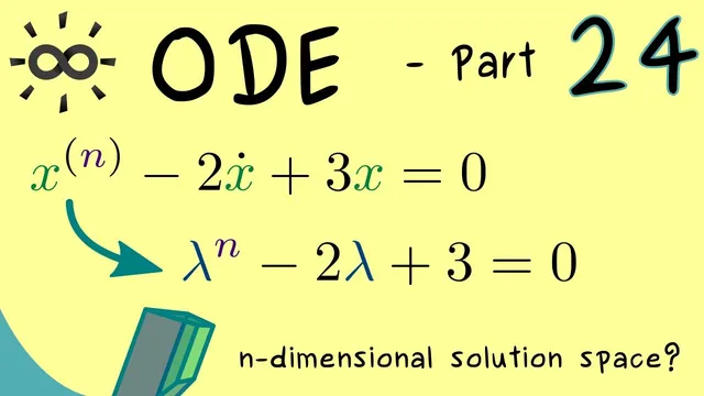
A practical memory aid reinforces this: test an exponential trial solution x(t) = e^{λt}. Plugging it into the ODE makes derivatives pull down powers of λ, reproducing the characteristic polynomial. Then the general solution follows from the roots. If A has n distinct real eigenvalues λ1,…,λn, A is diagonalizable, and the solution space is spanned by n exponential functions e^{λ_i t}. Returning from y to x uses the first component y1 = x, so the original nth-order ODE has a general solution that is a linear combination of those exponentials. When eigenvalues repeat or A is not diagonalizable over the reals, the zeros of the characteristic polynomial still come first—but additional cases must be handled in later discussions.