Ordinary Differential Equations 25 | Example for Non-Diagonalizable Matrix
Based on The Bright Side of Mathematics's video on YouTube. If you like this content, support the original creators by watching, liking and subscribing to their content.
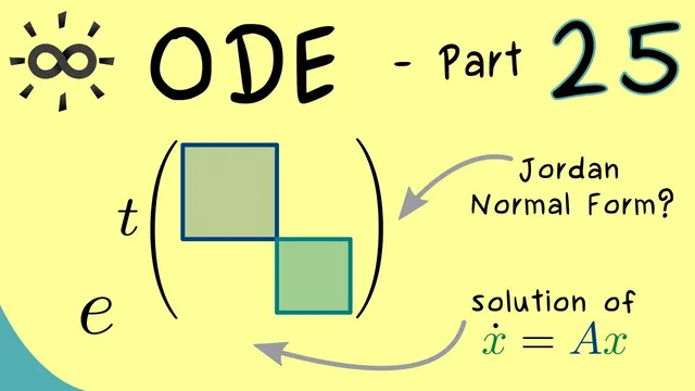
For ẋ = Ax with x(0)=x0, the unique solution is x(t)=e^{tA}x0, so computing e^{tA} is the central task.
Briefing
A system of linear differential equations with a non-diagonalizable matrix still has a closed-form solution once the matrix exponential is computed—by converting the matrix to Jordan normal form and exploiting the special structure of each Jordan block. With ẋ = Ax and an initial condition x(0)=x0, the unique solution is x(t)=e^{tA}x0, so the real task is calculating e^{tA} when A cannot be diagonalized.
The approach hinges on Jordan normal form: A is written as a block diagonal matrix whose blocks correspond to eigenvalues, with ones on the superdiagonal inside each block and zeros elsewhere. In the worked example, A is already in Jordan form with two Jordan blocks: one for eigenvalue 2 and one for eigenvalue 3. Even when blocks share the same size, their internal “box” structure differs, and that changes the polynomial factors that appear in e^{tA}.
For each Jordan block, the matrix exponential is computed by splitting the block into a diagonal part plus a nilpotent part. Concretely, for the Jordan block associated with eigenvalue 3 (a 3×3 block in the example), the block is decomposed as D+N, where D is diagonal (all 3’s on the diagonal) and N contains only the ones above the diagonal. The nilpotent matrix N satisfies N^2≠0 but N^3=0, so the exponential’s infinite power series collapses to a finite sum: e^{tN}=I+tN+(t^2/2)N^2. A key technical step is that D and N commute, which allows the factorization e^{t(D+N)}=e^{tD}e^{tN}. Since e^{tD} is just the exponential applied to each diagonal entry, the result becomes a triangular matrix with e^{3t} on the diagonal and additional terms like t e^{3t} and (t^2/2)e^{3t} in the superdiagonal positions.
The same method applies to the Jordan block for eigenvalue 2 (a smaller block in the example). Again, the block splits into a diagonal component and a nilpotent component. Here the nilpotent part squares to zero, so e^{tN} truncates after the linear term: e^{tN}=I+tN. Multiplying by e^{tD} produces another triangular matrix with e^{2t} on the diagonal and a t e^{2t} term in the appropriate superdiagonal entry.
Finally, the full matrix exponential e^{tA} is assembled by combining the exponentials of all Jordan blocks in the correct order. The takeaway is practical: even without diagonalizability, Jordan form turns e^{tA} into manageable algebra—triangular matrices whose entries are products of exponentials e^{λt} and low-degree polynomials in t determined by the size of each Jordan block.
Cornell Notes
For ẋ = Ax with x(0)=x0, the solution is x(t)=e^{tA}x0, so the main challenge is computing e^{tA} when A is not diagonalizable. Putting A into Jordan normal form breaks it into Jordan blocks, and each block can be written as D+N where D is diagonal (eigenvalue on the diagonal) and N is nilpotent (ones on the superdiagonal). Because D and N commute, e^{t(D+N)}=e^{tD}e^{tN}. Nilpotency makes e^{tN} a finite sum: for a block where N^3=0, e^{tN}=I+tN+(t^2/2)N^2. The resulting e^{tA} is block-diagonal (in Jordan form) with e^{λt} times polynomials in t, and assembling all blocks yields the full solution.
Why does the solution of ẋ = Ax reduce to computing a matrix exponential?
How does Jordan normal form make e^{tA} computable when A is not diagonalizable?
What is the D+N split inside a Jordan block, and why does it matter?
How does nilpotency turn the infinite exponential series into a finite sum?
What new terms appear in e^{tJ} for a Jordan block compared with a diagonalizable case?
Review Questions
- Given a Jordan block J = D+N with N^3=0, write the truncated form of e^{tN} and explain what determines the truncation point.
- How does the commuting condition between D and N enable the factorization e^{t(D+N)} = e^{tD}e^{tN}?
- Why do polynomial factors in t appear in e^{tA} for non-diagonalizable matrices, and how are they linked to Jordan block size?
Key Points
- 1
For ẋ = Ax with x(0)=x0, the unique solution is x(t)=e^{tA}x0, so computing e^{tA} is the central task.
- 2
Converting A to Jordan normal form reduces the problem to computing exponentials of individual Jordan blocks.
- 3
Each Jordan block can be written as J = D + N, where D is diagonal (eigenvalue on the diagonal) and N is nilpotent (ones on the superdiagonal).
- 4
Because D and N commute, e^{tJ} factors as e^{tD}e^{tN}, turning matrix exponential computation into two simpler exponentials.
- 5
Nilpotency forces e^{tN} to truncate to a finite polynomial in t, with the highest power determined by the smallest k such that N^k=0.
- 6
Assembling the block exponentials in the correct Jordan order yields the full e^{tA}, and the final solution follows by multiplying by x0.