Ordinary Differential Equations 4 | Reducing to First Order

TL;DR

An nth-order explicit ODE can be reduced to a first-order system by defining state variables as the function and its derivatives up to order n−1.

Briefing Cornell Notes

Briefing

Higher-order ordinary differential equations can be rewritten as first-order systems by packaging derivatives into a vector of state variables. That shift matters because it lets mathematicians apply the same first-order theory tools—like directional fields—and treat many different ODE forms within one unified framework.

The method starts with an explicit third-order example: the highest derivative is the third derivative of x, and it equals a function of lower derivatives and x itself. Concretely, the equation has the form x‴ = cos(x″) + (x′)² + x, with no time variable t appearing on the right-hand side, making it autonomous. To reduce it, define a vector y whose components are x and its derivatives: y1 = x, y2 = x′, and y3 = x″. Then the original third derivative x‴ becomes the first derivative of the third component, meaning y3′ = x‴. The right-hand side can be rewritten entirely in terms of y’s components as well: x″ = y3, x′ = y2, and x = y1. The remaining derivative relationships become extra equations that “connect” the components: y2′ = y3 and y1′ = y2. Together, these form a first-order system of three equations that contains exactly the same information as the original single third-order ODE. In compact form, the system can be written as y′ = V(y), where V is a vector-valued function.

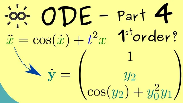
A second issue arises when the ODE is non-autonomous—when t appears explicitly on the right-hand side. Using a similar third-order structure but with a term like −t^4, the same derivative-to-vector trick still produces a first-order system, but it remains non-autonomous because t still shows up. The fix is to eliminate explicit t by treating time as an additional state variable. Introduce a new vector with one extra component, counting from y0 = t up through y3 = x″ (so the vector has four components). The original equation’s t-dependent term is rewritten as y0^4, making the system autonomous. To complete the transformation, add the trivial evolution equation for time: y0′ = 1. The result is an autonomous first-order system in one higher dimension.

In general terms, an autonomous nth-order ODE can be converted into a first-order autonomous system with n components in the state vector. If the original ODE is non-autonomous, the same construction yields an autonomous first-order system with n + 1 components by adding time as an extra variable. Solutions to the first-order system translate back to solutions of the original ODE through the definitions of the components (e.g., x = y1, x′ = y2, and so on). The practical takeaway is that restricting attention to the autonomous first-order system form is not a limitation; it’s a convenient normalization that covers both autonomous and non-autonomous ODEs.

Cornell Notes

Any explicit higher-order ODE can be rewritten as a first-order system by turning the unknown function and its derivatives into a vector of state variables. For an autonomous nth-order ODE, define y = (x, x′, …, x^(n−1)); then y′ = V(y) becomes a first-order autonomous system with n components. If the ODE is non-autonomous (t appears explicitly), add time as an extra state variable y0 = t, so the system becomes autonomous with n + 1 components, including the simple equation y0′ = 1. Solutions of the first-order system map back to solutions of the original ODE directly from the component definitions.

How does a third-order autonomous ODE become a first-order system?

Start with an equation like x‴ = cos(x″) + (x′)² + x. Define y1 = x, y2 = x′, y3 = x″. Then x‴ becomes y3′, and the right-hand side rewrites using y3, y2, and y1. The derivative links become y1′ = y2 and y2′ = y3. Together these give a first-order system for y = (y1, y2, y3).

Why does adding time as a new component make a non-autonomous ODE autonomous?

If t appears explicitly (e.g., x‴ = … − t^4), the first-order reduction still contains t on the right-hand side. By setting y0 = t and rewriting −t^4 as −y0^4, t no longer appears explicitly. The system becomes autonomous because the right-hand side depends only on the y-components. The added equation y0′ = 1 supplies the missing dynamics for time.

What changes in the state vector when moving from an autonomous nth-order ODE to a non-autonomous one?

For an autonomous nth-order ODE, the state vector has n components: (x, x′, …, x^(n−1)). For a non-autonomous ODE, time must be included as an extra component, so the state vector has n + 1 components: (t, x, x′, …, x^(n−1)).

How can a solution of the first-order system be converted back to a solution of the original ODE?

The component definitions provide the translation. If y1 = x, y2 = x′, and y3 = x″ (and similarly for higher order), then any solution y(t) of the first-order system immediately yields x(t) = y1(t). The original higher-order ODE is satisfied because the system was built to match the derivative relationships.

What is the compact form of the reduced autonomous system?

After reduction, the system can be written as y′ = V(y), where V is a vector-valued function built from the original ODE’s right-hand side. This form emphasizes that the evolution depends only on the current state y, not explicitly on time (once the non-autonomous case has been handled by adding y0 = t).

Review Questions

Given an autonomous fourth-order ODE, what state vector components should be used to reduce it to a first-order system?
If an ODE contains an explicit term like sin(t), how would you modify the state vector so the resulting first-order system becomes autonomous?
Why is it valid to treat the autonomous first-order system form as a general setting rather than a restriction?

Key Points

1
An nth-order explicit ODE can be reduced to a first-order system by defining state variables as the function and its derivatives up to order n−1.
2
For an autonomous nth-order ODE, the reduced system is autonomous and uses n state components: (x, x′, …, x^(n−1)).
3
For a non-autonomous ODE with explicit t-dependence, time is added as an extra state variable y0 = t to remove explicit t from the right-hand side.
4
Adding y0 = t requires the additional equation y0′ = 1, completing the autonomous first-order system.
5
The reduced first-order system contains exactly the same information as the original higher-order ODE because the derivative relationships are enforced component-by-component.
6
Solutions transfer back to the original ODE directly via the component definitions (e.g., x = y1, x′ = y2, etc.).

Highlights

A third-order ODE like x‴ = cos(x″) + (x′)² + x becomes a three-equation first-order system by setting y1 = x, y2 = x′, y3 = x″.

Non-autonomous terms such as −t^4 can be eliminated by introducing y0 = t, rewriting −t^4 as −y0^4, and adding y0′ = 1.

After reduction, autonomous first-order systems take the compact form y′ = V(y), where V depends only on the state vector y.

Treating only autonomous first-order systems is not a restriction: non-autonomous ODEs can always be converted into that form by expanding the state dimension.

Topics

Reducing ODE Order
First-Order Systems
Autonomous vs Non-Autonomous
State Vector Method
Solution Translation