Partial Differential Equations 1 | Introduction and Definition
Based on The Bright Side of Mathematics's video on YouTube. If you like this content, support the original creators by watching, liking and subscribing to their content.
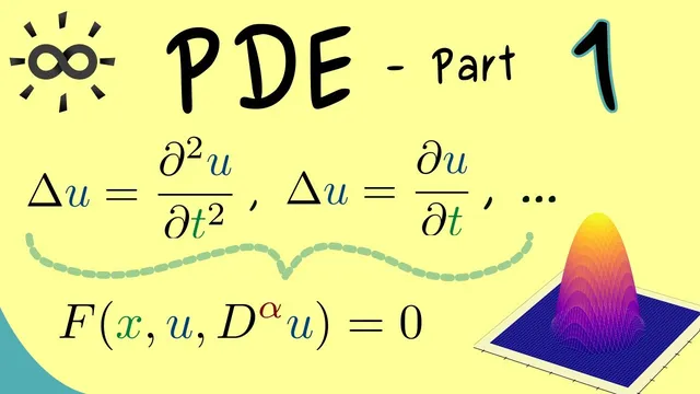
A PDE is an equation involving partial derivatives of an unknown function u(x) over a domain Ω ⊂ R^n, typically with n ≥ 2.
Briefing
Partial differential equations (PDEs) are introduced as the next step beyond ordinary differential equations: instead of derivatives with respect to a single variable, PDEs involve partial derivatives of an unknown function across a region of space. The central idea is that a PDE is an equation tying together values of an unknown function u(x) and its derivatives at each point x in a domain Ω ⊂ R^n (typically open, often connected). The “order” of a PDE is determined by the highest order of partial derivatives that appear—so if second derivatives are the highest ones involved, the PDE has order two.
The course frames PDEs through three canonical examples that already reveal why the same differential operator can behave very differently. All three examples use the Laplace operator (often written as Δ, called the “Laplacian”). The first is Laplace’s equation, which seeks solutions of Δu = 0. The second is the heat equation, which adds a first time derivative: it combines the Laplacian with ∂u/∂t, reflecting how heat diffuses over time. The third is the wave equation, which also starts with the Laplacian but adds a second time derivative on the other side, capturing oscillatory motion. These structural differences lead to a classification: Laplace’s equation is elliptic, the heat equation is parabolic, and the wave equation is hyperbolic.
After establishing these examples, the series sets up a general definition of what counts as a PDE. Formally, a PDE is described by a function f that takes a point x in Ω, the unknown value u(x), and a collection of partial derivatives of u at x. Multi-indices α organize which derivatives appear, and the maximum order m among them defines the PDE’s order. A key distinction is linearity: a PDE is linear if u and all its partial derivatives enter the equation in a linear way. That still allows coefficients depending on x (but not on u). The course also distinguishes homogeneous linear PDEs (with zero on the right-hand side) from inhomogeneous ones (with a nonzero term), noting that inhomogeneous equations can often be rewritten to move the right-hand side to the left.
Finally, the series defines a “classical solution.” A classical solution is a function u defined on the entire domain Ω such that all partial derivatives required by the PDE exist and are well-defined, and the PDE holds pointwise: the equation is satisfied for every x in Ω. The emphasis is practical—classical solutions match the familiar notion from ordinary differential equations—while also flagging that later in the course other solution concepts will be introduced when classical differentiability is too strict.
To prepare for the series, the course lays out prerequisites: multivariable calculus for partial derivatives and higher-dimensional integration, with measure theory and functional analysis treated as helpful but not strictly necessary at this stage. The overall roadmap is clear: learn the three benchmark PDE types first, then generalize toward more abstract tools (like function spaces and distributions) once the foundational definitions are in place.
Cornell Notes
The course introduces partial differential equations (PDEs) as equations involving partial derivatives of an unknown function u(x) over a domain Ω ⊂ R^n. A PDE’s order is the highest derivative order appearing (e.g., order 2 if second derivatives are included). Using the Laplace operator Δ, three benchmark equations illustrate how small structural changes produce different behaviors: Laplace’s equation is elliptic, the heat equation is parabolic (it includes ∂u/∂t), and the wave equation is hyperbolic (it includes a second time derivative). Linearity is defined by how u and its derivatives enter the equation, allowing x-dependent coefficients. A classical solution requires u to be differentiable enough so the PDE holds pointwise for every x in Ω.
What makes an equation a PDE rather than an ODE?
How is the order of a PDE determined?
Why do Laplace’s equation, the heat equation, and the wave equation get different classifications?
What does “linear PDE” mean in this framework?
What is a classical solution to a PDE?
What prerequisites are considered most important before studying PDEs?
Review Questions
- How does the highest derivative order in a PDE determine its classification as order m?
- What changes between Laplace’s equation, the heat equation, and the wave equation that lead to elliptic, parabolic, and hyperbolic types?
- What differentiability requirements distinguish a classical solution from weaker solution notions mentioned for later in the course?
Key Points
- 1
A PDE is an equation involving partial derivatives of an unknown function u(x) over a domain Ω ⊂ R^n, typically with n ≥ 2.
- 2
The order of a PDE equals the highest order of partial derivatives appearing in the equation.
- 3
Using the Laplace operator Δ, Laplace’s equation (Δu = 0) is elliptic, the heat equation is parabolic (includes ∂u/∂t), and the wave equation is hyperbolic (includes a second time derivative).
- 4
A linear PDE requires u and its derivative terms to enter the equation linearly, while coefficients may depend on x but not on u.
- 5
Homogeneous linear PDEs have zero on the right-hand side, while inhomogeneous linear PDEs include a nonzero forcing term that can be moved to the left.
- 6
A classical solution is a sufficiently differentiable function on Ω such that the PDE holds pointwise for every x ∈ Ω.
- 7
Multivariable calculus is the main prerequisite because it provides the partial derivative machinery PDEs rely on.