Probability Theory 16 | Variance
Based on The Bright Side of Mathematics's video on YouTube. If you like this content, support the original creators by watching, liking and subscribing to their content.
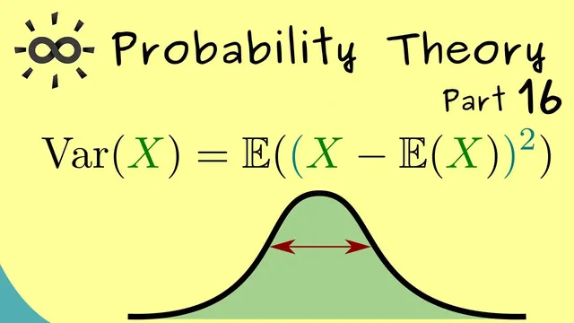
Variance quantifies spread around the expectation by averaging squared deviations: Var(X)=E[(X−E[X])²].
Briefing
Variance turns “how far from the mean” into a precise number. After expectation identifies the average location a random variable fluctuates around, variance measures the typical spread by quantifying how much the values deviate from that expectation—using a definition built to behave well mathematically.
The construction starts with the deviation random variable X − E[X]. This new quantity has expectation 0, but it can be positive or negative, so squaring it removes sign and focuses on magnitude. Variance is then defined as Var(X) = E[(X − E[X])²], assuming only that the relevant expectation exists (in particular, that E[X²] is finite). Because variance is itself an expectation, it inherits the same “average of a function” structure as expectation.
Expanding the square yields a more computationally convenient form. Writing (X − E[X])² = X² − 2E[X]·X + (E[X])², and using linearity of expectation plus the fact that E[c] = c for constants, the middle term simplifies and the final result becomes Var(X) = E[X²] − (E[X])². This version is often easier in practice: once E[X] is known, calculating variance reduces to finding E[X²] and subtracting the square of the mean.
For actual calculations, the transcript distinguishes between discrete and continuous settings. In the discrete case, expectations become sums over outcomes weighted by the probability mass function. In the continuous case, expectations become integrals weighted by the probability density function. The only change from the expectation formulas is that the integrand involves X² instead of X.
A first worked example uses a discrete uniform distribution with n equally likely outcomes x₁, …, xₙ, each having probability 1/n. The expectation becomes the arithmetic mean, often written as x̄. Plugging into the variance definition gives Var(X) = (1/n)·∑_{j=1}^n (xⱼ − x̄)², i.e., the average of squared deviations from the mean.
The second example is continuous: an exponential distribution with parameter λ. From earlier results, E[X] = 1/λ. To get variance, the key step is computing E[X²] via the integral ∫₀^∞ x² · λ e^{−λx} dx. Using integration by parts twice, the result is E[X²] = 2/λ². Subtracting (E[X])² = 1/λ² gives Var(X) = 1/λ².
Overall, variance emerges as the standard, well-behaved measure of spread: it is defined through squared deviations, simplifies to E[X²] − (E[X])², and produces concrete formulas for common distributions like the discrete uniform and the exponential.
Cornell Notes
Variance measures how widely a random variable spreads around its expectation. It is defined as Var(X)=E[(X−E[X])²], which requires the relevant expectation to exist (notably E[X²]). Expanding the square and using linearity of expectation gives the practical identity Var(X)=E[X²]−(E[X])², so variance is “mean of the square minus square of the mean.” For a discrete uniform distribution over n outcomes x₁,…,xₙ, variance becomes (1/n)∑(xⱼ−x̄)², the average squared deviation from the arithmetic mean. For an exponential distribution with rate λ, E[X]=1/λ and E[X²]=2/λ², yielding Var(X)=1/λ².
Why define variance using (X − E[X])² instead of just X − E[X]?
How does the variance identity Var(X)=E[X²]−(E[X])² come from the definition?
What changes when computing variance for discrete versus continuous random variables?
How is variance computed for a discrete uniform distribution over x₁,…,xₙ?
Why does the exponential distribution end up with Var(X)=1/λ²?
Review Questions
- Given Var(X)=E[(X−E[X])²], derive Var(X)=E[X²]−(E[X])² step by step using linearity of expectation.
- For a discrete uniform distribution on n outcomes, express Var(X) in terms of the outcomes x₁,…,xₙ and their mean x̄.
- For an exponential distribution with rate λ, compute Var(X) using E[X]=1/λ and the value of E[X²].
Key Points
- 1
Variance quantifies spread around the expectation by averaging squared deviations: Var(X)=E[(X−E[X])²].
- 2
Variance is well-defined when the needed expectation exists, especially E[X²].
- 3
A practical formula simplifies calculations: Var(X)=E[X²]−(E[X])².
- 4
In discrete settings, expectations become sums weighted by the probability mass function; in continuous settings, they become integrals weighted by the density.
- 5
For a discrete uniform distribution over x₁,…,xₙ, variance equals (1/n)∑_{j=1}^n (xⱼ−x̄)².
- 6
For an exponential distribution with parameter λ, E[X²]=2/λ², leading to Var(X)=1/λ².