Probability Theory 23 | Stochastic Processes

Stochastic processes are framed as a clean way to model randomness that evolves over time: they’re essentially random variables arranged in a sequence indexed by time. That simple structure matters because many real-world systems don’t just produce one random outcome—they change step by step, from biological growth to board games and other time-dependent phenomena.

The course begins with an intuitive definition. A stochastic process takes an index set of “time points” (often discrete, like natural numbers, or continuous, like real numbers) and assigns a random variable to each time point. All those random variables live on the same underlying sample space, so the randomness is consistent across time. Formally, one fixes a sample space Ω, chooses a time index set T, and defines a mapping X_t for each t in T. The collection (X_t)_{t∈T} is the stochastic process. When T is discrete, the result is a sequence of random variables across time steps; when T is continuous, it becomes a family of random variables across a continuum of times. In either case, the process can be viewed as a “path” traced by a particular outcome ω as time progresses.

To make the abstraction concrete, the transcript builds a coin-toss game designed to track when a specific pattern first appears: the first time two successive heads occur. The game runs indefinitely, and the random variable X_n is defined using three values—0, 1, and 2—based on the status after n tosses. After n tosses, if two successive heads have not yet occurred and the nth toss is tails (or the pattern hasn’t been achieved), the value is 0. If two successive heads still haven’t occurred but the nth toss is heads, the value is 1, capturing the “one heads in a row” partial progress. If two successive heads have occurred within the first n tosses, the value becomes 2. This middle value is crucial: it encodes the system’s memory of the most recent toss, which determines what can happen next.

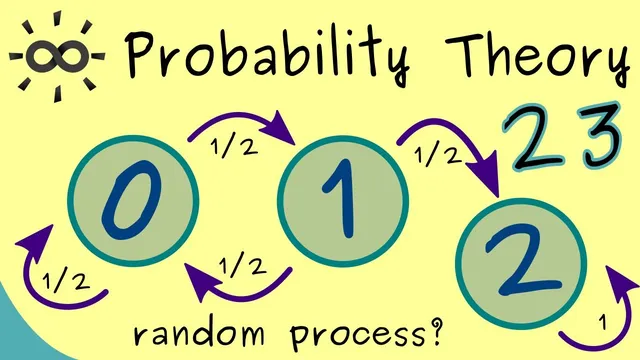
With the sample space Ω taken as the set of all infinite sequences of heads and tails, the transcript then translates the game into a dynamic state picture. From state 0, the next toss is heads with probability 1/2, moving the process to state 1; tails with probability 1/2 keeps it in state 0. From state 1, a heads outcome with probability 1/2 completes the pattern and moves to state 2, while tails with probability 1/2 resets progress back to state 0. Once state 2 is reached, the process is absorbing: it stays at 2 with probability 1, because the condition “two successive heads have occurred” remains true forever.

The takeaway is that stochastic processes turn pattern-based randomness into a time-evolving model with states and transition probabilities. The coin game illustrates how indexing by time, choosing a suitable sample space, and defining meaningful state values together produce a rigorous framework for analyzing systems that evolve under uncertainty.