Probability Theory 27 | kσ-intervals

TL;DR

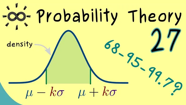
Define the kσ interval as [μ − kσ, μ + kσ], where μ = E[X] and σ = √Var(X].

Briefing Cornell Notes

Briefing

K-sigma intervals give a distribution-agnostic way to bound how much probability mass lies near the mean: for any random variable with finite expectation and variance, the probability of landing within μ ± kσ is at least 1 − 1/k². The key tool behind this guarantee is Chebyshev’s inequality, which turns variance information into a universal statement about deviations from the mean—no assumption of normality required.

Start with a random variable X whose expectation μ and variance σ² are finite. The kσ interval is defined as the set of outcomes where X stays within k standard deviations of the mean, i.e., X ∈ [μ − kσ, μ + kσ] (typically a closed interval). The question becomes: what is P(μ − kσ ≤ X ≤ μ + kσ)? Chebyshev’s inequality bounds the probability of large deviations, but it naturally targets events of the form |X − μ| > ε. Setting ε = kσ and converting to the complement yields the bound

P(|X − μ| ≤ kσ) ≥ 1 − Var(X)/ε² = 1 − σ²/(k²σ²) = 1 − 1/k².

This estimate is weak for k = 1 (it becomes non-informative), but it becomes meaningful for k ≥ 2. For k = 2, the lower bound is 1 − 1/4 = 3/4, so at least 75% of outcomes fall inside the “two sigma” interval. For k = 3, the bound becomes 1 − 1/9 = 8/9, meaning at least about 88.9% of outcomes lie within μ ± 3σ.

The universality matters: these percentages hold for any distribution with finite variance, even if the true probability could be much higher. The normal distribution is the benchmark case where the actual coverage is far better than Chebyshev’s guarantee. For a standard normal variable (μ = 0, σ = 1), the familiar empirical/known probabilities are approximately 68% within 1σ, about 95% within 2σ, and about 99.7% within 3σ.

To illustrate the improvement over Chebyshev’s bound, the transcript describes a simulation in R using the standard normal distribution (via Norm). By drawing n samples (e.g., 1,000), then counting the fraction that fall between −k and +k, the observed proportions cluster around the classic normal-rule values: roughly 68% for k = 1, around 95% for k = 2, and near 99% for k = 3, converging toward 99.7% as sample size grows. The takeaway is practical: Chebyshev provides a conservative, distribution-free safety net, while the normal distribution delivers much tighter concentration around the mean—especially for the 1σ/2σ/3σ intervals that recur throughout statistics.

Cornell Notes

K-sigma intervals define a “near the mean” region for any random variable with finite mean μ and variance σ²: X ∈ [μ − kσ, μ + kσ]. Using Chebyshev’s inequality with ε = kσ and taking complements gives a universal lower bound: P(|X − μ| ≤ kσ) ≥ 1 − 1/k². This bound is non-useful for k = 1, but it guarantees at least 75% coverage for k = 2 and at least 8/9 (≈88.9%) for k = 3, regardless of the distribution. For the normal distribution, actual coverage is much higher—about 68% (1σ), 95% (2σ), and 99.7% (3σ)—which can be confirmed via simulation in R. These numbers are widely used in statistics because they reflect how tightly normal data concentrates around μ.

How is a kσ interval defined, and what does it mean operationally?

A kσ interval is the set of values where the random variable stays within k standard deviations of its mean: [μ − kσ, μ + kσ]. Operationally, it asks for the probability mass of outcomes whose X-values fall in that band around μ (typically using a closed interval). The scale is set by σ, the square root of Var(X), so the interval adapts to the spread of the distribution.

What universal probability guarantee comes from Chebyshev’s inequality for kσ intervals?

Chebyshev’s inequality bounds deviations of the form P(|X − μ| > ε) ≤ Var(X)/ε². Choosing ε = kσ and converting to the complement gives P(|X − μ| ≤ kσ) ≥ 1 − Var(X)/(k²σ²) = 1 − 1/k². This holds for any real-valued random variable with finite expectation and variance, regardless of its distribution shape.

Why does the Chebyshev bound fail to be informative at k = 1?

Plugging k = 1 into 1 − 1/k² yields 1 − 1 = 0. A lower bound of 0 does not rule out anything beyond what probabilities already guarantee, so it provides no meaningful concentration information for the “one sigma” interval in the distribution-free setting.

What coverage guarantees does Chebyshev’s inequality give for k = 2 and k = 3?

For k = 2, the bound is 1 − 1/4 = 3/4, so at least 75% of outcomes lie in μ ± 2σ. For k = 3, the bound is 1 − 1/9 = 8/9, so at least about 88.9% lie in μ ± 3σ. These are conservative guarantees that apply even to heavy-tailed or skewed distributions, as long as variance is finite.

How does the normal distribution compare to Chebyshev’s conservative bounds, and how is it checked in practice?

For a standard normal variable (μ = 0, σ = 1), the actual probabilities are much higher: about 68% within 1σ, about 95% within 2σ, and about 99.7% within 3σ. The transcript describes simulating n samples from Norm in R, then computing the fraction that fall between −k and +k (e.g., between −1 and +1 for 1σ). Increasing n reduces fluctuation and makes the simulated fractions approach the classic normal values.

Review Questions

What lower bound does Chebyshev’s inequality give for P(|X − μ| ≤ kσ), and how does it depend on k?
Why is the Chebyshev-based estimate for the 1σ interval not useful in the distribution-free setting?
In a simulation of a standard normal distribution, what fraction of samples should fall within μ ± 3σ, and why does increasing sample size improve the estimate?

Key Points

1
Define the kσ interval as [μ − kσ, μ + kσ], where μ = E[X] and σ = √Var(X].
2
Chebyshev’s inequality converts variance information into a bound on deviation probabilities from the mean.
3
For any distribution with finite mean and variance, P(|X − μ| ≤ kσ) is at least 1 − 1/k².
4
The distribution-free Chebyshev bound is non-informative for k = 1 because it yields a lower bound of 0.
5
Chebyshev guarantees at least 75% coverage for k = 2 and at least 8/9 (≈88.9%) coverage for k = 3.
6
Normal data concentrates far more tightly than Chebyshev predicts: about 68% (1σ), 95% (2σ), and 99.7% (3σ).
7
Monte Carlo simulation in R can estimate these normal-interval coverages by sampling from Norm and counting values within ±k.

Highlights

Chebyshev’s inequality yields a clean, distribution-free guarantee: P(|X − μ| ≤ kσ) ≥ 1 − 1/k².

Even without assuming normality, the two-sigma interval must contain at least 75% of probability mass.

For the normal distribution, the classic 68% / 95% / 99.7% rule shows how much tighter concentration can be than Chebyshev’s conservative bounds.

Simulation confirms the normal interval coverages by sampling from a standard normal and measuring the fraction within ±k standard deviations.

Topics

K-Sigma Intervals
Chebyshev’s Inequality
Standard Deviation
Normal Distribution
Monte Carlo Simulation

Mentioned

R
P
Var
E
E[X]