Probability Theory 28 | Weak Law of Large Numbers

The weak law of large numbers formalizes a simple but powerful idea: when independent, identically distributed random outcomes are sampled many times, the observed relative frequency of an event gets close to its theoretical probability. The key point isn’t that the relative frequency converges perfectly every time; it’s that the chance of a noticeable deviation becomes small as the number of trials grows. In the coin-toss example, the fraction of heads among the first n tosses behaves like a random variable whose probability of differing from 1/2 by more than any fixed ε shrinks toward zero as n increases—capturing why large samples reliably reflect underlying probabilities.

To make that connection precise, the discussion distinguishes theoretical probability from empirical probability (relative frequency). The theoretical side comes from a probability measure P on a model space, while the empirical side comes from repeatedly running the experiment and counting how often outcomes fall in an event A. For n tosses, the empirical probability of heads can be written as a random variable: define Xk to be 1 if the k-th toss is heads and 0 otherwise, then the relative frequency is X̄n = (1/n)∑_{k=1}^n Xk. Because X̄n is itself random, “convergence” must be defined in a probabilistic sense.

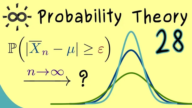
That probabilistic convergence is given by convergence in probability. The weak law of large numbers says that X̄n converges in probability to μ, where μ is the common expected value of the underlying i.i.d. variables. Concretely, for every ε>0, the probability that the relative frequency deviates from μ by at least ε, namely P(|X̄n−μ|≥ε), tends to 0 as n→∞. This is the operational meaning of “the empirical probability approaches the theoretical probability” without requiring almost-sure (path-by-path) convergence.

The assumptions needed for the general statement are spelled out: the random variables must be independent and identically distributed (IID), and their expectations must exist in a way that ensures integrability—expressed as E(|X1|)<∞. Under these conditions, μ = E(X1) is also the expectation of every Xk and of the average X̄n.

A clean proof route is then given for the common special case where the variables have finite variance. Let Var(X1)=Σ^2. Using expectation properties, the average still has mean μ. Using variance properties and independence, the variance of the average scales down like Var(X̄n)=Σ^2/n. Chebyshev’s inequality then turns that variance shrinkage into a probability bound: P(|X̄n−μ|≥ε) ≤ Var(X̄n)/ε^2 = Σ^2/(nε^2). Since Σ^2 and ε are fixed, the right-hand side goes to 0 as n grows, forcing the deviation probability to vanish—exactly the weak law’s convergence-in-probability claim. The result hinges on finite variance; the next step is to consider how things change when variance assumptions fail, which is left for a later application-focused discussion.