Probability Theory 30 | Strong Law of Large Numbers
Based on The Bright Side of Mathematics's video on YouTube. If you like this content, support the original creators by watching, liking and subscribing to their content.
The weak law of large numbers gives convergence in probability: P(|X̄_n − μ| ≥ ε) → 0 for every ε > 0.
Briefing
The strong law of large numbers upgrades the usual “average settles down” message by guaranteeing point-by-point convergence of sample averages—not just that large deviations become unlikely. For independent, identically distributed (IID) random variables with a finite expected value, the running average converges to the common mean almost surely, meaning it happens for all outcomes except a probability-zero set. This matters because it matches how repeated random experiments behave when the underlying outcome ω is fixed: the long-run average should stabilize for almost every ω, not merely for most ω in aggregate.
The starting point is the weak law of large numbers, which uses convergence in probability. Under the weak law, for any ε > 0, the probability that the sample average differs from the mean by at least ε goes to zero as the number of samples n grows. Formally, that means the probability measure of the set of outcomes where |X̄_n(ω) − μ| ≥ ε shrinks to nothing as n → ∞. But this framework doesn’t guarantee what happens at a specific ω over time. A fixed ω can still exhibit “bad” behavior at infinitely many n values—even if the set of ω that are bad at a given n becomes small—so the weak law alone can’t rule out persistent outliers across different sample sizes.
The strong law addresses that gap by switching from probability-based statements about sets of outcomes to an almost sure statement about the limit itself. With an IID sequence (X_k) and an integrability condition (the expectation of |X_k| is finite, so the mean exists), the sample average X̄_n(ω) converges to μ as n → ∞ for almost every ω. “Almost surely” is made precise by probability: the set of outcomes where convergence fails has probability exactly one complement, i.e., probability zero. So while exceptions are logically possible, they are confined to a null set.
A key relationship links the two laws: almost sure convergence is stronger than convergence in probability. Consequently, once the strong law holds under the stated IID and integrability assumptions, the weak law follows automatically. That’s why the strong law is often treated as the more informative result: it delivers the stabilization of averages for essentially every realized sequence of outcomes, not just in the sense of shrinking deviation probabilities.
Finally, the discussion notes that the assumptions can be adjusted in other formulations of the strong law, but the common practical version remains centered on IID random variables with finite expectation. Under those conditions, both the strong and weak law of large numbers are available together, providing a robust foundation for why averages of random quantities become reliable in the long run. The next step is to move toward limit theorems beyond the law of large numbers.
Cornell Notes
For IID random variables with a finite mean μ, the sample average X̄_n converges to μ as n → ∞ in an almost sure sense. “Almost surely” means the set of outcomes ω where convergence fails has probability 0, so the stabilization happens for essentially every realized sequence. This is stronger than the weak law, which only guarantees convergence in probability: for any ε > 0, the probability that |X̄_n − μ| ≥ ε goes to 0 as n grows. Because almost sure convergence implies convergence in probability, the strong law automatically yields the weak law under the same IID and integrability assumptions. The distinction matters because the weak law alone doesn’t rule out infinitely many “bad” sample sizes along a fixed ω.
What exactly does the weak law guarantee, and what does it fail to guarantee for a fixed outcome ω?
How does the strong law strengthen the conclusion?
What assumptions are used for the strong law in this presentation?
Why does proving almost sure convergence automatically give convergence in probability?
What does “almost surely” mean in terms of probability measure?
Review Questions
- In what sense does convergence in probability differ from almost sure convergence for the sequence of sample averages X̄_n(ω)?
- Why can the weak law still allow infinitely many deviations along a fixed ω, even though P(|X̄_n − μ| ≥ ε) → 0?
- Under what conditions on an IID sequence does the strong law guarantee X̄_n(ω) → μ almost surely?
Key Points
- 1
The weak law of large numbers gives convergence in probability: P(|X̄_n − μ| ≥ ε) → 0 for every ε > 0.
- 2
Convergence in probability does not ensure that a fixed outcome ω eventually stays within any ε-neighborhood of μ.
- 3
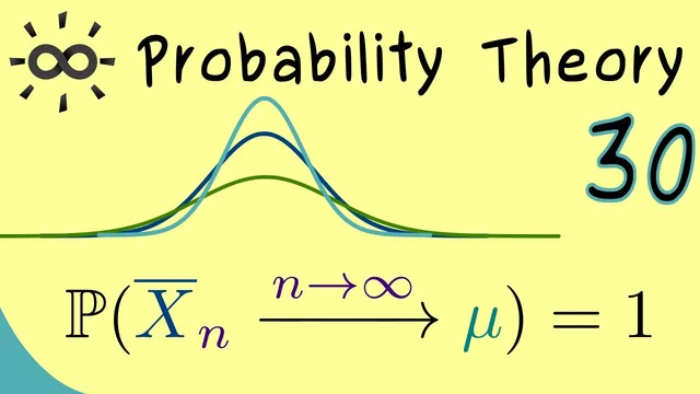
The strong law of large numbers gives pointwise stabilization: X̄_n(ω) → μ as n → ∞ for almost every ω.
- 4
“Almost surely” means the set of outcomes where convergence fails has probability 0 (probability one for the good set).
- 5
For IID random variables with finite expectation (integrability), the strong law holds and therefore the weak law follows automatically.
- 6
Almost sure convergence is strictly stronger than convergence in probability, which is why the strong law implies the weak law.