Probability Theory 31 | Central Limit Theorem

Central limit theorem assumptions are simple—independent, identically distributed random variables with finite mean and variance—and they drive a powerful payoff: standardized sample averages become approximately normal, and in the limit they converge to the standard normal distribution. This matters because it turns complicated averaging behavior into a predictable bell curve, enabling practical approximations for uncertainty and fluctuations in real-world data.

Start with IID random variables X1, X2, …, Xn. The distribution of each Xi can be anything, as long as the expectation E[X1] = μ and the variance Var(X1) = σ² exist and are finite. The sample mean X̄n = (1/n)∑_{k=1}^n Xk inherits the same expectation as the individual variables, so E[X̄n] = μ. But its variance shrinks with sample size: Var(X̄n) = σ²/n. Larger n means smaller fluctuations around μ, a theme already familiar from the law of large numbers—yet the central limit theorem goes further by describing the *shape* of those fluctuations.

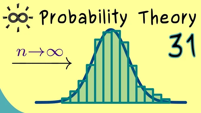
A concrete example uses an urn model without replacement, connected to the hypergeometric distribution: five balls contain two types, and three are drawn; each random variable counts how many “ones” appear in the draw. The expectation for that count is given as 9/5 (about 1.8). By simulating many such draws and plotting histograms of X̄n for different n values, the distribution of the sample mean tightens around 1.8 as n grows. More importantly, the histogram begins to resemble a bell curve. Increasing n makes the approximation to normality clearer, while the spread decreases in line with the 1/n variance scaling.

The theorem’s formal statement comes from standardizing the sample mean. Define a standardized variable

YN = ( (X̄n − μ) / (σ/√n) ).

This transformation shifts the mean to 0 and rescales the variance to 1. Under the IID and finite-mean/finite-variance conditions, the distribution of YN converges to the Normal(0,1) distribution as n → ∞. One way to express this convergence is through cumulative distribution functions: for each real x, the CDF of YN, P(YN ≤ x), approaches the CDF of the standard normal. That limiting CDF can be written as an integral of the standard normal density from −∞ to x, using the familiar exponential form exp(−t²/2).

A key takeaway is robustness: the original Xi distribution doesn’t need to be normal. As long as the variables are IID and have finite expectation and variance, averages become approximately normal for large n, which explains why Gaussian models appear so often in statistics and applied probability.