Probability Theory 33 | Descriptive Statistics (Sample, Median, Mean)

TL;DR

Descriptive statistics summarizes what’s already observed in a finite sample, while inductive statistics uses those summaries to infer properties of a larger population under uncertainty.

Briefing Cornell Notes

Briefing

Statistics shifts the focus from modeling random experiments to extracting information from a fixed set of observations. Within that broader field, descriptive statistics summarizes what’s already in the data, while inductive (influential) statistics uses those summaries to infer properties of a larger, unseen population—an inference that must be expressed probabilistically because uncertainty remains.

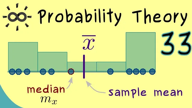
A key starting point is the sample: a finite collection of real numbers (or, more generally, vectors in R^d) drawn from a much larger set of possible outcomes. If each observation is a real number, the sample can be written as an ordered tuple (X1, X2, …, Xn). Ordering matters because it enables direct visualization and definitions like the median. For small samples, points on a number line can be arranged from left to right; for larger samples, a histogram becomes more practical. A histogram groups values into intervals (“boxes”) along the x-axis and counts how many observations fall into each interval.

Those counts lead to two related frequency concepts. The absolute frequency of a subset A of R is the number of sample elements XK that lie in A. Because absolute counts can be large, descriptive statistics also uses relative frequency, obtained by dividing the absolute frequency by the sample size n. Relative frequencies fall between 0 and 1 and provide a normalized picture of how often values occur—without claiming anything probabilistic about the underlying population.

To compress the entire sample into a single representative number, descriptive statistics uses measures of central tendency. The sample mean (often written as X̄) is the arithmetic average: add all observations and divide by n. The mean reflects the “center” of the data, but it is sensitive to outliers; moving one extreme value can pull the mean noticeably.

The median (written as M(X)) offers a more robust alternative. After sorting the data, the median is the middle observation. For an odd n, it is the value at index (n+1)/2. For an even n, there is no single middle point, so the median is defined as the average of the two central values (indices n/2 and n/2 + 1). This definition makes the median depend only on how many points lie on each side, not on how far any single point is from the center.

Finally, descriptive statistics addresses spread with the (unbiased) sample variance, denoted s_X^2. It measures how far observations typically deviate from the sample mean by summing squared differences (XK − X̄)^2 and applying a normalization factor of 1/(n−1). The “unbiased” choice is designed so the sample variance can serve as an estimator for the variance of the underlying probability distribution—setting up the transition from description to induction in later discussions.

Cornell Notes

Descriptive statistics summarizes a finite sample of observations—real numbers or vectors in R^d—using tools that compress the data into understandable quantities. A sample can be visualized with a histogram, where absolute frequency counts how many observations fall in a subset A and relative frequency divides those counts by n. Central tendency is captured by the sample mean X̄ (the arithmetic average) and the median M(X), the middle value after sorting (or the average of the two middle values when n is even). Spread is measured by the unbiased sample variance s_X^2, computed from squared deviations from the mean with normalization 1/(n−1). These definitions matter because they provide the building blocks for later inductive statistics, where summaries help estimate properties of an unseen population.

What is a “sample” in descriptive statistics, and how does it differ from the larger population idea?

A sample is a finite set of observations—mathematically, an ordered tuple (X1, X2, …, Xn). Each observation is a real number (or, in R^d, a vector). The sample is treated as a small selection drawn from a much larger set of possible data (the population). Descriptive statistics then summarizes only what’s in this finite set, without claiming full knowledge of the population.

How do absolute and relative frequency connect to histograms?

Given a subset A of R (an interval/“box” on the x-axis), the absolute frequency f_abs(A) is the number of sample points XK that lie in A. The histogram’s bar height corresponds to this count (or, equivalently, the number of indices k with XK ∈ A). Relative frequency is f_rel(A) = f_abs(A)/n, producing a value between 0 and 1 that normalizes for sample size.

Why can the sample mean be misleading when outliers exist?

The sample mean X̄ is computed as (1/n)∑_{k=1}^n Xk. Because it uses every data point with equal weight, shifting one extreme observation far away changes the sum and therefore moves X̄. In contrast, the median depends only on the rank order and the number of points on each side, not on the magnitude of an outlier.

How is the median defined for odd versus even sample sizes?

After sorting the sample, if n is odd, the median is the middle observation at index (n+1)/2, which in the example with n=15 corresponds to X8. If n is even, there is no single middle point, so the median is defined as the average of the two central values at indices n/2 and n/2 + 1 (a “virtual” middle value).

What does the unbiased sample variance measure, and why use 1/(n−1)?

The unbiased sample variance s_X^2 measures spread by summing squared deviations from the sample mean: ∑_{k=1}^n (Xk − X̄)^2, then normalizing. The normalization factor is 1/(n−1), not 1/n, because this choice makes the estimator unbiased for the variance of the underlying probability distribution (a point reserved for later deeper discussion).

Review Questions

When constructing a histogram, what changes when the partition of the x-axis into intervals becomes finer?
For n even, which two indices determine the median, and how is the median computed from them?
Write the conceptual steps for computing the unbiased sample variance from a sample and indicate what role the sample mean plays.

Key Points

1
Descriptive statistics summarizes what’s already observed in a finite sample, while inductive statistics uses those summaries to infer properties of a larger population under uncertainty.
2
A sample is a finite ordered tuple (X1, …, Xn); each observation can be a real number or a vector in R^d.
3
Absolute frequency counts how many observations fall into a subset A of R; relative frequency divides that count by n to normalize between 0 and 1.
4
The sample mean X̄ is the arithmetic average and is sensitive to outliers because every data point affects the sum.
5
The median M(X) is the middle value after sorting; for even n it is the average of the two central observations, making it more robust to extreme values.
6
The unbiased sample variance s_X^2 quantifies spread using squared deviations from the mean and uses normalization 1/(n−1) to support unbiased estimation of the underlying variance.

Highlights

Relative frequency is built directly from histogram counts by dividing absolute frequency by the sample size n, producing values between 0 and 1.

The median’s definition changes for odd versus even n: it’s the single middle observation for odd n, but the average of the two central values for even n.

The unbiased sample variance uses normalization 1/(n−1), positioning it as an estimator for the variance of the underlying probability distribution.

The mean can shift dramatically when one observation is moved far from the rest, while the median depends only on ranks.

Topics

Descriptive Statistics
Sample Mean
Median
Histogram Frequencies
Sample Variance