Probability Theory 34 | Statistical Model

TL;DR

Inferential statistics selects a parameter θ from a family of candidate probability measures P_θ because finite samples can match infinitely many distributions.

Briefing Cornell Notes

Briefing

Inferential (inductive) statistics starts with a simple but stubborn fact: a finite sample can be produced by infinitely many probability distributions. The core task is therefore not to “discover” a single distribution from data, but to choose the most plausible member of a whole family of candidate distributions. Concretely, a sample is treated as coming from an underlying random variable X, but the same observed outcomes can match many different probability laws. That ambiguity is handled by introducing a parameterized collection of probability measures P_θ indexed by θ in a parameter space Θ. The statistical goal becomes selecting the best-fitting θ—while keeping Θ large enough to avoid throwing away relevant possibilities, yet small enough to make the mathematics workable.

A key modeling step is deciding what family P_θ to use. The transcript illustrates this with a normal-distribution example: assume the data come from a normal distribution with variance fixed at 1, while the mean is unknown. In that setup, θ is the mean, and each candidate distribution P_θ is fully determined by that single parameter. Even the parameter space can be restricted for practical reasons—such as limiting plausible mean values to a range like −5 to +5—so the model reflects prior knowledge about where measurements should land. Once the family is fixed, the remaining question is how to pick the “most suitable” θ given an observed sample.

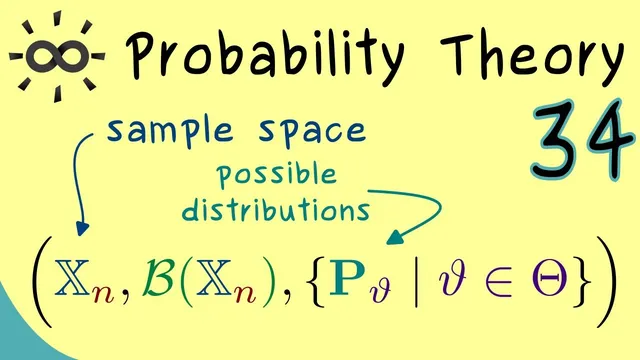
To formalize the sample, the transcript distinguishes between the probability-theory notion of a random variable and the statistics notion of a sample space. For a sample of size n (with dimension d simplified to 1), the sample space is a subset X_N of R^n, meaning every observed dataset must lie in X_N. The sample itself can be viewed as the outcome of n random variables X_1, …, X_n. Because each data point comes from the same measurement process, these random variables are modeled as independent and identically distributed (iid): they share the same distribution and differ only by realization.

With these pieces in place, the definition of a statistical model is introduced. A statistical model fixes (1) the sample space X_N, (2) a family of distributions P_θ, and (3) the way those distributions apply to n observations via the n-fold product measure P_θ^N. This product-measure construction enables probabilities for subsets of X_N. The transcript also notes the use of the appropriate σ-algebra (BL σ-algebra on X_N) to make the probability assignments mathematically precise. In short, a statistical model is the resulting collection of probability spaces—one for each θ—built to support inference.

Finally, the framework sets up the next stage: estimating θ from data. The transcript flags two main inference tools—point estimators and interval estimators—leaving the detailed methods for the following video.

Cornell Notes

Inferential statistics treats an observed dataset as evidence about an unknown parameter θ inside a family of candidate probability distributions P_θ. Because the same finite sample can arise from infinitely many distributions, the model is built by choosing a parameter space Θ and restricting attention to distributions indexed by θ. A common example assumes a normal distribution with variance fixed at 1, leaving only the mean θ unknown; even Θ can be narrowed using prior knowledge (e.g., plausible mean values). The sample of size n is formalized as points in a sample space X_N ⊆ R^n, modeled as n iid random variables X_1,…,X_n. A statistical model then consists of the n-fold product measures P_θ^N on X_N, enabling probability statements about subsets and setting up estimation of θ.

Why can’t inference uniquely determine the underlying distribution from a finite sample?

A finite sample is only a finite set of outcomes, and many different probability distributions can generate the same sample outputs. That means the data alone don’t pin down a single distribution; instead, inference must compare a whole family of plausible distributions and choose the parameter θ that makes the observed data most consistent with that family.

How does the normal-distribution example turn an unknown distribution into a parameterized family P_θ?

The model assumes the data come from a normal distribution with variance fixed at 1, while the mean is unknown. The mean becomes the parameter θ, so each θ corresponds to a specific probability measure P_θ: a normal distribution centered at θ with variance 1. Restricting θ to a range (like −5 to +5) further narrows the candidate distributions to those considered realistic.

What is the difference between a random variable’s sample space in probability theory and a sample space in statistics?

In probability theory, a random variable X is defined on an abstract sample space ω. In statistics, the “sample space” X_N refers to the set of all possible observed datasets of size n, i.e., X_N ⊆ R^n. The notation may overlap (both use X), but context distinguishes whether it means an abstract probability-theory space or the set of possible data vectors.

Why model X_1,…,X_n as iid?

Each entry in the sample is produced by the same measurement process. That assumption implies the random variables representing each observation should not differ in distribution; they are independent realizations of the same underlying random variable. This is captured by the iid assumption: independent and identically distributed.

What does the n-fold product measure P_θ^N accomplish in defining a statistical model?

The transcript starts with P_θ as a probability measure on R (for a single observation). To model n observations jointly, it constructs the n-fold product measure P_θ^N, which assigns probabilities to subsets of X_N ⊆ R^n. This step is what turns a one-dimensional distribution family into a family of joint distributions for datasets.

What inference problem is set up after defining the statistical model?

Once the family of models (indexed by θ) is fixed, the remaining task is to estimate θ from the observed sample. The transcript previews two categories of estimation: point estimators (a single best value for θ) and interval estimators (a range of plausible θ values), with interval methods reserved for the next video.

Review Questions

In what sense does the choice of parameter space Θ affect whether a statistical method is feasible and informative?
Given a sample of size n modeled as iid random variables, what role does the product measure P_θ^N play in computing probabilities for datasets?
Why is restricting θ to a smaller range (like −5 to +5) considered part of building a statistical model rather than a later step?

Key Points

1
Inferential statistics selects a parameter θ from a family of candidate probability measures P_θ because finite samples can match infinitely many distributions.
2
A good parameter space Θ balances two competing needs: it must be mathematically manageable and also broad enough not to discard relevant possibilities.
3
Modeling choices—such as assuming a normal distribution with fixed variance—convert an unknown distribution into a parameterized family indexed by θ.
4
A dataset of size n is formalized as a point in a sample space X_N ⊆ R^n, and the sample is modeled as outcomes of n random variables X_1,…,X_n.
5
Assuming iid observations encodes the idea that each data point comes from the same measurement process.
6
A statistical model is built by combining the sample space X_N with the family of n-fold product measures P_θ^N on X_N, enabling probability statements about subsets.
7
The next inference step is estimating θ, using either point estimators or interval estimators.

Highlights

Finite samples don’t identify a unique distribution; inference instead chooses the best θ inside a parameterized family P_θ.

Fixing variance at 1 in a normal model turns the unknown mean into the parameter θ, making the candidate distributions concrete.

The sample space in statistics is the set of all possible data vectors X_N ⊆ R^n, distinct from the abstract ω used to define random variables.

Modeling n observations requires the n-fold product measure P_θ^N, which supports joint probability assignments to subsets of X_N.

A statistical model is essentially a collection of probability spaces indexed by θ, setting up estimation of θ from data.

Topics

Inferential Statistics
Statistical Models
Parameter Space
iid Sampling
Product Measures