Recurrent Neural Networks (RNN) - Deep Learning w/ Python, TensorFlow & Keras p.7
Based on sentdex's video on YouTube. If you like this content, support the original creators by watching, liking and subscribing to their content.
RNNs are designed for tasks where the order of inputs carries meaning, such as time series and natural language.
Briefing
Recurrent neural networks (RNNs) are built for problems where order matters—especially time series and natural language—because the meaning of a sequence depends on what came before. Instead of treating inputs as independent features, an RNN feeds each step of the sequence into a recurrent cell and carries information forward to the next step. That “memory” is what lets the model distinguish between sentences that share words but differ in order, such as “some people made a neural network” versus “a neural network made some people,” where word order changes the interpretation.
The core mechanism is implemented through recurrent cells, most commonly LSTM (long short-term memory) units. An LSTM cell receives (1) the current input at a time step and (2) information passed from the previous time step, then decides what to forget, what new information to add, and what to output. In practice, each time step produces outputs that can feed forward to the next layer and/or to the next recurrent step. The transcript also notes that architectures can be extended to bidirectional recurrent layers, where information flows in more than one direction through the sequence.
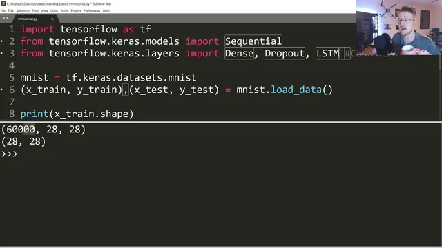
After laying out the intuition, the tutorial shifts to a practical goal: building a simple RNN from scratch using TensorFlow/Keras. The main challenge isn’t the model code—it’s shaping data into sequences with targets. To keep things easy, the example uses the MNIST dataset and treats each 28×28 image as a sequence of 28 rows, where each row is a time step. That means the model sees 28 steps per sample, each step containing 28 pixel values.
The model is assembled as a Keras Sequential network with stacked LSTM layers (128 units in the first LSTM, then another LSTM with 128 units). Because the second recurrent layer needs the full sequence, the first LSTM uses return_sequences=True. Dropout layers are added to reduce overfitting, followed by dense layers: a 32-unit dense layer and a final dense layer with 10 outputs using softmax for digit classification.
Training initially runs poorly and slowly, with accuracy not improving and loss not trending downward. The transcript identifies a key issue: the input images weren’t normalized to the 0–1 range. After scaling X_train and X_test by dividing by 255, learning accelerates dramatically and accuracy climbs quickly. The tutorial also highlights performance differences between LSTM implementations: switching to the GPU-optimized “CuDNNLSTM” (with tanh-based behavior) yields much faster epochs and reaches strong validation performance within the same number of epochs.
By the end, validation accuracy reaches about 98% while training accuracy is slightly lower, which is attributed to how Keras reports metrics (training accuracy averaged across an epoch versus validation measured at the end). The takeaway is that RNNs can be straightforward to run when data is already sequential, but preprocessing—especially normalization—can make the difference between a model that barely learns and one that converges quickly. The next step promised is a more realistic time-series example that will require heavier preprocessing.
Cornell Notes
Order-sensitive tasks are where recurrent neural networks shine: each time step’s output depends on earlier steps. LSTM cells implement this “memory” using gates that decide what to forget, what to add, and what to output, and they can pass information both forward to later layers and onward to the next time step. The tutorial demonstrates a simple MNIST setup by treating each 28×28 image as a sequence of 28 rows (each row is one time step). A stacked LSTM model with dropout and dense layers is trained with sparse categorical cross-entropy and softmax output. The biggest practical lesson is normalization: dividing pixel values by 255 turns a slow, non-learning run into fast convergence; using CuDNNLSTM further speeds training on GPU.
Why does word order or time order matter to an RNN, and how is that different from a standard feedforward network?
What does an LSTM cell do at each time step?
How did the tutorial convert MNIST images into a sequence suitable for an RNN?
Why did training accuracy and loss look wrong at first, and what fixed it?
What is the practical difference between LSTM and CuDNNLSTM in this setup?
Why can validation accuracy be higher than training accuracy in Keras logs?
Review Questions
- When building an RNN for sequence data, what does return_sequences=True control, and why would a second recurrent layer require it?
- How does dividing inputs by 255 change the training dynamics, and what symptoms in the logs would suggest normalization is missing?
- In the MNIST-as-sequence approach, what exactly is the “time step,” and what is the feature vector at each step?
Key Points
- 1
RNNs are designed for tasks where the order of inputs carries meaning, such as time series and natural language.
- 2
LSTM cells maintain sequence information using gates that decide what to forget, what to add, and what to output at each time step.
- 3
A simple RNN example can be built by reshaping MNIST images into sequences of 28 rows, treating each row as one time step.
- 4
Normalization is critical: scaling pixel values to the 0–1 range (divide by 255) can turn a non-learning run into fast convergence.
- 5
Stacked LSTM layers often require return_sequences=True in earlier LSTM layers so later layers receive the full sequence.
- 6
Using CuDNNLSTM can dramatically speed up training on GPU compared with a standard LSTM configuration.
- 7
Validation accuracy can exceed training accuracy when training metrics are averaged over an epoch but validation is computed at the epoch’s end.