Session 44 - Confidence Intervals | DSMP 2023

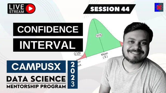
Confidence intervals are presented as the practical fix for a simple problem: a single sample statistic (like the sample mean) can’t reliably pin down an unknown population parameter. Instead of claiming a precise number, confidence intervals give a range that is tied to a confidence level—most commonly 95%—so the unknown population mean is expected to fall inside that range in repeated sampling. The session builds this idea from first principles, starting with population vs. sample, then moving through point estimation, and finally deriving how the interval is calculated.

The walkthrough begins with core statistical foundations. Population is the full set of interest (e.g., all students), while a sample is a random subset used because studying everyone is impossible. Parameters describe population quantities (often denoted with Greek letters), while statistics describe sample quantities. Since parameters are typically unknown, inference uses sample data to estimate them. This naturally leads to inferential statistics, where the goal is to make predictions or decisions about population characteristics using limited samples.

From there, “point estimate” is introduced as a single-number summary of the population parameter—most often the sample mean. The instructor uses an analogy: if someone predicts an exact cricket score and is paid only when the prediction is exactly correct, that level of certainty is unrealistic because the true outcome varies. Confidence intervals replace that unrealistic exactness with a probabilistic range.

The session then defines confidence intervals as ranges constructed around the point estimate using a margin of error. The margin of error depends on (1) the confidence level (through a critical value), (2) the population standard deviation (or an estimate of it), and (3) the sample size. The confidence level is clarified to avoid a common misunderstanding: it does not mean the population mean has a 95% probability of lying in the interval for a single computed interval. Instead, it means that if the sampling-and-interval-building process were repeated many times, about 95% of the constructed intervals would contain the true population parameter.

Two calculation procedures are taught. The z-procedure applies when the population standard deviation is known and the sampling assumptions hold; it uses the standard normal critical value (z) and typically relies on the Central Limit Theorem when sample size is large (the instructor emphasizes n ≥ 30). The t-procedure is introduced for the more realistic case where the population standard deviation is unknown. It replaces the z critical value with a t critical value from the t-distribution, which accounts for extra uncertainty via “degrees of freedom” (n − 1). As degrees of freedom increase, the t distribution approaches the normal distribution, making the t-procedure converge toward the z-procedure.

Finally, the session emphasizes how interval width changes with inputs: higher confidence levels widen intervals (larger margin of error), larger population variability widens intervals, and larger sample sizes narrow them—especially when moving from small to moderate sample sizes. A practical example with a YouTube-style dataset (CampusX subscribers) and a discussion of a prior Titanic-related implementation mistake reinforce the idea that the correct standard deviation must be used in the right place (sampling distribution vs. sample-level variability), otherwise the confidence interval coverage can be wrong. The class ends by previewing next steps: hypothesis testing, then regression and machine learning topics, with confidence intervals serving as a foundational tool for inference.