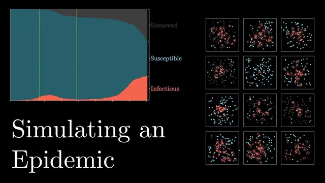
Simulating an epidemic

Epidemic control in these simulations hinges less on dramatic, late interventions and more on catching infectious people early and reliably. In an agent-based SIR setup—where people move randomly, infection happens when susceptible agents spend time within an “infection radius” of infectious ones, and infectious agents eventually recover—the epidemic can explode quickly, infecting nearly everyone in short order. Small parameter changes produce outsized effects: doubling the infection radius (more interactions) drives the system to a sharp, near-simultaneous peak, while halving the per-contact infection probability (better hygiene) spreads the curve out substantially.

The model also makes a practical point about healthcare capacity: if the peak is too high, mortality rises because systems get overwhelmed. That connects to a recurring real-world feature—people don’t just wander; they converge on shared destinations like schools or markets. Introducing a central location that agents regularly visit can raise the epidemic’s intensity dramatically, pushing the basic reproductive number (R0) as high as 5.8 in the simulation. Even when social distancing is turned on, keeping the central destination active can blunt its benefits, leaving total cases close to the control scenario.

The strongest lever remains identification and isolation of infectious cases. Once the simulation hits a threshold number of cases, infectious agents are removed from the general population one day after infection—standing in for rapid quarantine. Under perfect detection, the epidemic stops quickly. But “leaky” detection changes the story: if 20% of infectious people slip through because they show no symptoms and avoid testing, the peak rises only slightly while a long tail emerges, doubling total infections and prolonging the outbreak. With 50% isolated, outcomes barely improve compared with doing nothing, because enough infectious agents keep seeding new infections.

These dynamics intensify when multiple communities are connected by travel. Cutting travel rates can help in some runs—sometimes leaving entire communities unscathed—but the effect is inconsistent once infection is already present. In larger “cities,” concentrated hubs accelerate spread: once infection reaches a central urban area, it quickly reaches other hubs and then slowly works its way outward.

To quantify spread, the simulations track the effective reproductive number (R), estimating how many secondary infections each infectious person generates over their infectious period. R greater than 1 marks exponential growth (an epidemic), around 1 indicates endemic persistence, and below 1 signals decline. The model’s R values shift sharply with assumptions: R peaks around 2.2 in the baseline, rises to about 8 when infection radius doubles, and sits around 1.3–1.7 when infection probability halves. For comparison, COVID-19’s R0 is cited as a little above 2, while seasonal flu is around 1.3.

Social distancing still matters, especially for flattening the curve, but imperfections prolong transmission. When 100% of agents avoid close contact, the outbreak dies out; when only 70% or 90% comply, total infections remain only modestly reduced and the tail lasts longer. The simulations ultimately argue for layered control: early testing, fast isolation, and effective treatment (modeled as moving people out of the infectious category) outperform reliance on behavior changes alone. If people relax measures while infectious cases remain uncontrolled, the model warns of a second wave—particularly in a world with travel and shared hubs.