Simulating and understanding phase change | Guest video by Vilas Winstein

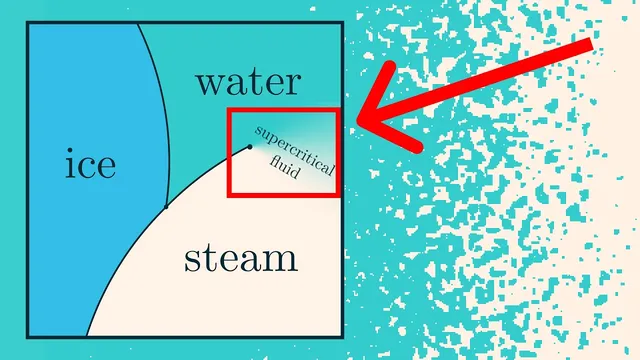
A discretized “liquid–vapor” model reproduces water-like phase behavior—complete with a liquid–gas phase transition, a supercritical region, metastability, and fractal structure at the critical point—using only a simple energy rule plus statistical mechanics. The key insight is that macroscopic phases emerge from a competition between energy minimization (favoring clumped molecules) and entropy maximization (favoring many disordered configurations). That balance shifts with temperature, and the model’s phase diagram in the (temperature, chemical potential) plane mirrors the qualitative shape of real water.

The simulation represents a box as a grid of pixels: blue pixels hold molecules, white pixels are empty space. Two parameters steer the system. Temperature controls how strongly energy matters relative to randomness. Pressure is hard to implement directly in a fixed-size grid, so the model uses chemical potential instead, which plays a role analogous to pressure by controlling the tendency for the number density to increase or decrease. At high temperature, density changes smoothly with chemical potential—matching the idea of a supercritical fluid where liquid and gas become continuously connected. At low temperature, the system abruptly switches between low-density (gas-like) and high-density (liquid-like) behavior, producing a phase transition line; during the transition, the grid separates into regions that are mostly liquid-like or gas-like rather than smoothly blending.

Under the hood, the model samples microstates using the Boltzmann distribution: each configuration’s probability is proportional to exp(−E/T), where E is the microstate energy. The video motivates this formula by starting from isolated systems where all microstates at fixed energy are equally likely, then coupling two systems and asking what quantity equalizes at equilibrium. The equalized derivative of entropy with respect to energy is 1/T, which leads directly to exp(−E/T) when a small system is placed in a large heat bath at temperature T.

To make the phase transition happen in a tractable way, the energy function is deliberately simple: molecules prefer to be adjacent, with each neighboring pair lowering energy (implemented as −1 per adjacent pair, and 0 otherwise). At low temperature, the energy advantage of forming a dense droplet beats the entropy loss from restricting configurations. At high temperature, entropy dominates, so dispersed “gas” configurations win.

Efficient sampling requires more than writing down the distribution. Instead of enumerating exponentially many microstates, the simulation uses Markov chain Monte Carlo via Kawasaki Dynamics: repeatedly propose local moves that conserve molecule count (swap a molecule between two pixels) and accept them with probabilities determined by the Boltzmann weight ratio exp(−ΔE/T). Allowing molecule number to fluctuate leads to a grand-canonical version controlled by chemical potential, enabling larger, GPU-friendly simulations by proposing add/remove moves per pixel.

Beyond the phase diagram, the model shows physically familiar phenomena. Droplets and bubbles expand only after crossing the transition line far enough to overcome kinetic “kick” requirements; otherwise the system can linger in the metastable gas phase until a sufficiently large droplet forms. At the critical point, density patterns become self-similar fractals with scale invariance. The same underlying lattice physics maps onto the Ising model (liquid/gas ↔ spin up/down) and, with continuous spin directions, onto the XY model with vortices. Finally, the video emphasizes universality: many microscopic details can change without destroying the qualitative macroscopic behavior, which is why simplified models can still capture the essence of real phase transitions.