Solving the heat equation | DE3

The heat equation’s solutions aren’t determined by the differential equation alone: the temperature profile must satisfy the PDE in the rod’s interior and also obey boundary conditions that encode how heat behaves at the ends. That distinction matters because even functions that satisfy the heat equation can evolve in physically wrong ways if they ignore what happens at x = 0 and x = L.

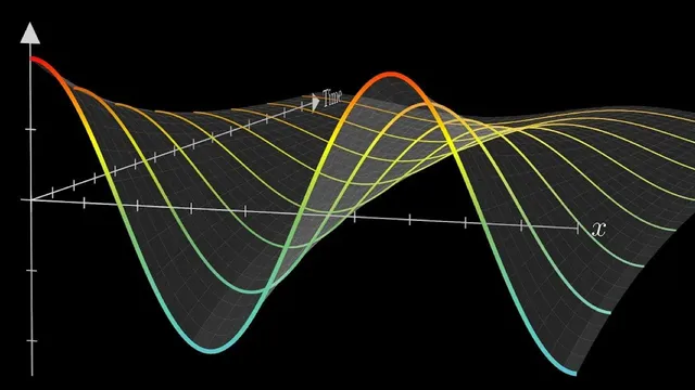
In one dimension, the heat equation links time change to spatial curvature: the rate of temperature change at a point is proportional to the second derivative of temperature with respect to position. This creates a natural search for “nice” spatial shapes. Fourier’s key move was to treat the problem like an orchestra of modes: sine waves are simple building blocks because their second spatial derivatives reproduce the same shape (up to a constant factor). Starting with an idealized initial profile T(x,0) = sin(x), the second derivative in x turns sin(x) into −sin(x), so the PDE reduces to an exponential-in-time scaling. That leads to a candidate solution of the form T(x,t) = sin(x)·e^{−αt}, where α is the proportionality constant in the heat equation. Checking derivatives confirms it satisfies the PDE: differentiating twice in space brings down a negative factor, while differentiating once in time brings down the same factor times −α.

But the story breaks when physical boundary behavior is imposed. A straight-line temperature profile (proportional to x) has zero second derivative in space, so it would seem to stay constant under the PDE. Yet a simulation that models the ends correctly shows it slowly flattens toward a uniform temperature. The culprit is the boundary: at the rod’s ends there’s no neighbor on one side, so the “curvature drives change” intuition must be modified. For insulated ends—no heat flowing in or out—the slope at both endpoints must be zero for all times after the start. In mathematical terms, ∂T/∂x must vanish at x = 0 and x = L.

To satisfy those Neumann-type boundary conditions, sine waves need adjustment. Using cosine instead of sine shifts the wave so it’s flat at x = 0. The remaining task is to tune the spatial frequency so the derivative also vanishes at x = L. Introducing a factor ω inside the cosine changes the second derivative by ω², which forces the time-decay rate to pick up the same ω² factor: sharper spatial variation decays faster, with decay proportional to ω². The lowest allowed frequency occurs when ω = π/L, and higher modes come from harmonics—whole-number multiples of π/L—plus the constant mode (ω = 0). This produces an infinite family of functions that satisfy both the PDE and the insulated-end boundary conditions.

The payoff is strategic rather than final: once these mode solutions are in hand, the next step is to combine them to match arbitrary initial temperature distributions. The heat equation becomes solvable by decomposing complex starting shapes into sums of sine/cosine modes whose time evolution is exponential, with rates set by the spatial frequencies and the boundary constraints.