Taylor series | Chapter 11, Essence of calculus

Taylor series turn local derivative information at a single point into accurate polynomial approximations nearby—often so accurate that, when enough terms are added, the approximation becomes an infinite series equal to the original function. That “derivatives at one point → values near that point” pipeline matters because it replaces hard-to-handle functions (like trig and logs) with polynomials that are easier to compute, differentiate, and integrate, which is why Taylor methods show up across physics and engineering.

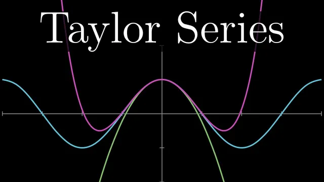
The core example builds a quadratic approximation to cos(x) near x = 0. Start with the most basic requirement: the polynomial must match the function’s value at the expansion point. Since cos(0) = 1, the constant term must be c0 = 1. Next comes the slope. The derivative of cos(x) is −sin(x), which is 0 at x = 0, so the quadratic’s linear coefficient must be chosen so the approximation also has a flat tangent there. That forces c1 = 0. Finally, the curvature: cos(x) has a negative second derivative at x = 0 because the second derivative of cos(x) is −cos(x), giving −1 at the origin. Matching the quadratic’s second derivative (which equals 2c2) yields c2 = −1/2. The result is the small-angle approximation cos(x) ≈ 1 − x^2/2, which already predicts cos(0.1) extremely well.

The same logic scales to higher-degree polynomials by matching higher derivatives. Adding a cubic term c3x^3 would require the third derivative at x = 0 to match that of cos(x). But the third derivative of cos(x) is sin(x), which equals 0 at x = 0, so c3 must be 0—meaning the quadratic is also the best possible cubic approximation. Adding a quartic term works differently: the fourth derivative of cos(x) is cos(x), which equals 1 at x = 0, so the coefficient must be 1/24. That produces 1 − x^2/2 + x^4/24, a polynomial that stays very close to cos(x) for small x.

A key structural takeaway is why factorials appear. When taking n derivatives of x^n, power-rule cascades produce factors 1·2·…·n, so the coefficient of x^n must be the nth derivative value divided by n! to “cancel out” that growth. Another crucial property: adding higher-order terms doesn’t disturb the lower-order matching at x = 0, because every extra term contains powers of x that vanish when evaluating derivatives at the expansion point. This is why each derivative order at x = 0 is controlled by exactly one coefficient.

General Taylor polynomials formalize the pattern: for an expansion about x = a, the coefficient of (x − a)^n is f^(n)(a)/n!. The video then connects the second-order term to geometry via the fundamental theorem of calculus by approximating how the area-under-a-curve function changes, where the quadratic term corresponds to a triangular area involving the second derivative. Stopping after finitely many terms gives Taylor polynomials; adding infinitely many terms gives Taylor series. Some series converge to the function everywhere (e^x, and also sine/cosine), while others converge only within a limited interval (ln x around x = 1), defining a radius of convergence. The unifying intuition is that derivative data at one point can be “propagated” into an approximation around that point—sometimes indefinitely, sometimes only up to a boundary.