The medical test paradox, and redesigning Bayes' rule

An accurate medical test can still produce a surprisingly low chance that a positive result is truly correct—because disease prevalence and the test’s false positives reshape what “accuracy” means for an individual. Using a breast-cancer screening example with 1% prevalence, 90% sensitivity, and 91% specificity, the test correctly flags 9 out of 10 women with cancer but also produces 89 false positives among 990 women without cancer. When a woman tests positive, the probability she actually has cancer becomes 9/(9+89) ≈ 1 in 11. The paradox is that the test is “over 90% accurate” in the usual sense, yet its positive predictive value (PPV) can be arbitrarily low when the disease is rare.

The counterintuitive gap shows up in real-world reasoning. In 2006–2007, psychologist Gerd Gigerenzer ran statistics seminars for practicing gynecologists using the same numbers as the breast-cancer scenario: prevalence around 1%, sensitivity 90%, specificity 91%. Many doctors answered that a positive result implies something like a 9-in-10 chance of cancer—far off the correct 1-in-11. The mismatch isn’t a logical contradiction; it’s a “veridical paradox,” meaning the facts are provably true but feel wrong when people treat test accuracy as if it directly converts into personal risk.

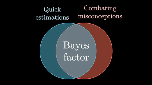
The fix starts with reframing what tests do. Rather than delivering a final probability, a test updates a prior—the baseline chance of disease before seeing results. In the example, the prior is 1 in 100. The test doesn’t replace that with 90% certainty; it shifts it to about 1 in 11, roughly an order-of-magnitude change. That updating strength can be summarized by a Bayes factor (also called a likelihood ratio), computed for a positive result as sensitivity divided by the false positive rate. Here, 0.9 / 0.09 = 10. A practical rule follows: multiply the prior odds by the Bayes factor.

Odds make the mathematics feel less like a trap. Prior odds are the number with cancer divided by the number without it; after a positive test, those odds are scaled by the Bayes factor. With 1% prevalence, prior odds are 1:99; multiplying by 10 yields 10:99, which converts back to about 1 in 11. If prevalence rises to 10%, prior odds become 1:9; after multiplying by 10, the result is 10:9, or roughly 53%—matching what a concrete population count predicts. The same logic works for negative results too, using a different factor: false negative rate divided by specificity (about 1 in 9 in the example), which reduces prior odds by about an order of magnitude.

Finally, the discussion contrasts the odds-and-Bayes-factor version of Bayes’ rule with the more common probability form. The odds framing cleanly separates prior information from test accuracy, making it easier to swap priors and chain multiple pieces of evidence (like symptoms or multiple tests). The standard formula remains valuable as a compact representation of the sample-population counting method, but the odds approach reduces ambiguity—especially because a Bayes factor is not a probability and therefore can’t be mistaken for “the chance your result is false.”