The other way to visualize derivatives | Chapter 12, Essence of calculus

TL;DR

Derivatives can be interpreted as local stretching, squishing, and flipping factors describing how a function transforms nearby inputs.

Briefing Cornell Notes

Briefing

Calculus intuition often gets trapped in graphs—slopes for derivatives, areas for integrals—but that graph-first mindset can make later topics feel like a conceptual cliff. A “transformational” view of derivatives reframes them as local stretching, squishing, and flipping factors when a function maps inputs on one number line to outputs on another. That shift matters because it generalizes cleanly to settings where you can’t easily draw the object you’re differentiating, such as multivariable calculus, complex analysis, and differential geometry.

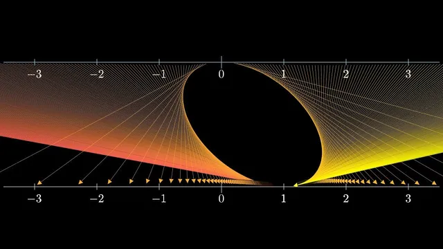
In the standard picture, the derivative at a point is the slope of the graph there. The alternate picture treats a function as a transformation: zoom in around an input x, look at nearby points, and see how their spacing changes after applying the function. For example, with f(x)=x^2, inputs near 1 get stretched by about a factor of 2, matching f′(1)=2. Near 3, the local stretching factor becomes about 6, consistent with f′(3)=6. When the derivative is between 0 and 1, the transformation contracts; when it is 0, the zoomed-in neighborhood collapses toward a point in the limit. Negative derivatives introduce a flip: near negative inputs for x^2, the local behavior resembles multiplying by a negative factor, meaning nearby points reverse orientation as well as change spacing. The key takeaway is that the derivative’s magnitude controls how strongly nearby points are pulled together or pushed apart under repeated application.

That local “density change” idea becomes concrete in a classic infinite fraction puzzle: 1 + 1/(1 + 1/(1 + 1/(…))). A common approach sets the expression equal to x and uses the self-similarity to solve a fixed-point equation. That equation has two solutions: the golden ratio φ≈1.618 and another value, −0.618 (equal to −1/φ). At first glance, the infinite fraction seems incompatible with a negative answer because every partial expression is positive. But the deeper question is what happens when the defining transformation is iterated.

Define the transformation T(x)=1+1/x. Starting from any seed value, repeatedly applying T generates a sequence that numerically converges to φ. Even seeds near −0.618 drift away and eventually jump back to φ. The stability explanation comes from the derivative of T at the fixed points. Near φ, the transformation contracts neighborhoods: |T′(φ)| is less than 1 (the transcript gives about 0.38 in magnitude), so perturbations shrink each iteration, pulling iterates back toward φ. Near −0.618, the derivative’s magnitude exceeds 1, so perturbations grow; the fixed point repels nearby values, making it unstable. In dynamical-systems language, φ is a stable fixed point and −0.618 is unstable.

Whether −0.618 should be accepted as “the” value depends on interpretation—limit versus algebraic fixed-point solution—but the iteration behavior strongly suggests φ is the meaningful limit for the infinite fraction. The broader lesson is not that graphs are wrong; it’s that treating derivatives as local transformation factors makes the concept more portable, especially when calculus moves beyond simple graphable functions.

Cornell Notes

The derivative can be understood not just as a graph slope, but as a local transformation factor: zoom in near an input x, apply the function, and measure how nearby points stretch, shrink, or flip. For f(x)=x^2, the derivative f′(x) gives the approximate scaling of spacing between nearby inputs after mapping. This viewpoint becomes powerful when iterating a function and studying fixed points. For the infinite fraction defined by T(x)=1+1/x, there are two fixed points (φ≈1.618 and −0.618), but only φ attracts nearby starting values. Stability is determined by whether |T′(fixed point)| is less than 1 (stable) or greater than 1 (unstable).

How does the “transformational” view of derivatives differ from the usual “slope” view?

Instead of treating f′(x) as the slope of a graph, the transformational view treats f as a mapping between number lines. Zoom in around an input x and look at a small cluster of nearby inputs; after applying f, the cluster’s spacing changes. The derivative f′(x) is the local factor describing that change: values with |f′(x)|<1 contract nearby points, |f′(x)|>1 expands them, and a negative derivative flips the neighborhood’s orientation. The slope picture is one special way to interpret sensitivity; the transformation picture is a more general way to interpret local behavior.

For f(x)=x^2, what does f′(1)=2 mean in the transformational picture?

The function sends 1→1, 2→4, 3→9, and so on. In the transformational picture, zoom in around x=1 and track where nearby points land. Near 1, the outputs spread out roughly by a factor of 2 compared with the input spacing. That local stretching factor is exactly what f′(1)=2 encodes: the closer the zoom, the more the mapping looks like multiplying by 2.

Why does the infinite fraction converge to φ rather than to −0.618, even though both are fixed points?

Both φ and −0.618 satisfy the fixed-point equation x=1+1/x, so each remains unchanged under one application of T(x)=1+1/x. But convergence depends on stability. Near φ, the transformation contracts neighborhoods because |T′(φ)|<1 (the transcript gives about 0.38 in magnitude). Near −0.618, |T′(−0.618)|>1, so small deviations grow and the iteration repels away from that fixed point. Iterating from typical seeds therefore drifts toward φ.

What is the stability criterion for fixed points in this setting?

A fixed point is stable if perturbing the input slightly makes the iterates return toward the fixed point. In this one-dimensional iteration, that stability is determined by the derivative’s magnitude: if |T′(x*)|<1 at the fixed point x*, nearby points get scrunched back toward x* each iteration; if |T′(x*)|>1, nearby points get stretched away and the fixed point is unstable. The sign of T′(x*) indicates whether neighborhoods flip, but the magnitude controls attraction versus repulsion.

How does the transformational view handle cases where a graph intuition is hard to use?

When calculus moves beyond functions that are easy to graph, the “zoom and measure local stretching/squishing” idea still applies. Even if the function’s output can’t be visualized as a simple curve, the derivative still describes how the mapping changes small neighborhoods. That’s why the transcript frames this as a bridge to multivariable calculus, complex analysis, and differential geometry: the derivative remains a local transformation descriptor even when graph-based intuition becomes awkward.

Review Questions

In the transformational view, what do the sign and magnitude of f′(x) tell you about what happens to a tiny neighborhood around x under f?
For T(x)=1+1/x, why can two fixed points exist while only one is reached by iterating from most starting values?
How does the condition |T′(x*)|<1 relate to the idea of “scrunching” neighborhoods under repeated application?

Key Points

1
Derivatives can be interpreted as local stretching, squishing, and flipping factors describing how a function transforms nearby inputs.
2
The magnitude |f′(x)| controls whether nearby points contract (|f′(x)|<1) or expand (|f′(x)|>1) under the mapping.
3
A negative derivative indicates a flip in orientation of a neighborhood, even when the magnitude determines stability.
4
For the infinite fraction, iterating T(x)=1+1/x reveals two fixed points—φ≈1.618 and −0.618—but only φ is stable.
5
Fixed-point stability in one-dimensional iteration is determined by whether |T′(fixed point)| is less than 1 (stable) or greater than 1 (unstable).
6
The “infinite fraction” value depends on interpretation: algebraic fixed points exist in both cases, but the limiting process selects the stable one.
7
Thinking of derivatives as transformation behavior makes the concept more transferable to calculus settings where graph intuition breaks down.

Highlights

The derivative’s real job in the transformational view is to measure how a function changes the spacing of nearby points when you zoom in.

For T(x)=1+1/x, both φ≈1.618 and −0.618 satisfy the fixed-point equation, yet iteration converges to φ because it attracts neighborhoods.

Stability comes down to a simple inequality: |T′(x*)|<1 pulls iterates in, while |T′(x*)|>1 pushes them away.

Negative derivatives don’t just change size—they reverse orientation of local neighborhoods.

The same local “zoom” idea that explains f′(1)=2 for x^2 also predicts which fixed point an infinite fraction selects.

Topics

Transformational View of Derivatives
Fixed Points and Stability
Infinite Fraction Iteration
Local Stretching and Flipping
Golden Ratio Convergence