The quick proof of Bayes' theorem

TL;DR

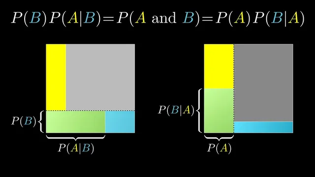
Bayes’ theorem can be derived by writing the same joint probability P(A and B) in two ways: P(A)·P(B|A) and P(B)·P(A|B).

Briefing Cornell Notes

Briefing

Bayes’ theorem can be justified with a short, purely mathematical identity built from how “AND” works in probability. For two events, A and B, the probability that both happen can be written two ways: P(A and B) = P(A)·P(B|A) and also P(A and B) = P(B)·P(A|B). Since both expressions describe the same joint probability, they must be equal. Rearranging gives the familiar Bayes’ theorem relationship, letting one conditional probability be expressed in terms of the other. The practical payoff is straightforward: when it’s easier to estimate P(evidence|hypothesis) than P(hypothesis|evidence), this identity turns that asymmetry into a usable calculation.

That “AND” breakdown also clarifies why Bayes’ theorem matters most in situations where events are not independent. A common mistake is to treat P(A and B) as P(A)·P(B) even when the events are correlated. The transcript highlights a heart-disease example: if 1 in 4 people die of heart disease, it’s tempting to multiply 1/4 by 1/4 and conclude the chance that both you and your brother die of heart disease is 1/16. The multiplication rule only works when the events are independent—when knowing A doesn’t change the probability of B. In real life, siblings share genetics and lifestyle factors, so if your brother dies of heart disease, your risk is no longer the baseline 1 in 4. In probability terms, P(B|A) is higher than P(B), so P(A and B) cannot be computed by simply multiplying marginals.

The contrast with coin flips and dice rolls is instructive. Those classic classroom examples are set up so that each event is independent of the last, which makes P(B|A) = P(B) and makes the clean multiplication intuition correct. But the most interesting probability problems—especially those that motivate Bayes’ theorem—are precisely the ones where dependence and correlation are the point. Bayes’ theorem is designed to quantify that dependence: it measures how strongly one variable’s probability shifts when new evidence about another variable arrives. That’s why the theorem isn’t just a rearrangement of symbols; it’s a tool for updating beliefs in the presence of real-world linkage between events.

Cornell Notes

Bayes’ theorem follows quickly from the fact that the joint probability P(A and B) can be written in two equivalent ways: P(A)·P(B|A) and P(B)·P(A|B). Setting these equal and rearranging yields a relationship that converts one conditional probability into the other. This matters because in many applications it’s easier to estimate “evidence given a hypothesis” than “a hypothesis given evidence.” The transcript also warns against a frequent misconception: multiplying P(A)·P(B) to get P(A and B) only works under independence. When events are correlated—like siblings’ health risks—P(B|A) differs from P(B), so the simple product rule fails.

How does the identity P(A and B) = P(A)·P(B|A) lead to Bayes’ theorem?

Start with two events A and B. The probability both occur can be expressed as P(A and B) = P(A)·P(B|A), because you can think of selecting cases where A happens (proportion P(A)) and then, within those, the fraction where B also happens (proportion P(B|A)). The same joint probability can also be written as P(A and B) = P(B)·P(A|B). Since both equal the same quantity, set them equal and rearrange to solve for the desired conditional probability (e.g., P(A|B) in terms of P(B|A), P(A), and P(B)).

Why does Bayes’ theorem often help when one conditional probability is easier to estimate than the other?

The two conditional probabilities in Bayes’ theorem are asymmetric: P(evidence|hypothesis) versus P(hypothesis|evidence). In many real problems, evidence models are more direct (for example, how likely a test result is if a condition is true), while the posterior probability of the condition given the test result is what people actually want. Bayes’ theorem uses the identity from the joint probability to translate between these two directions of conditioning.

What misconception leads people to compute P(A and B) as P(A)·P(B) even when it’s wrong?

The misconception is treating the product of marginals as the joint probability without checking independence. The transcript’s heart-disease example shows the trap: if 1 in 4 people die of heart disease, multiplying 1/4 by 1/4 suggests a 1/16 chance that both you and your brother die of heart disease. That assumes your brother’s outcome doesn’t affect your risk, but genetic and lifestyle links mean your risk changes after observing your brother’s death.

How does correlation show up in probability notation?

Correlation means dependence: P(B|A) is not equal to P(B). Under independence, P(B|A) = P(B), so P(A and B) = P(A)·P(B) becomes valid. When events are linked, conditioning on A changes the probability of B, so the correct joint probability must use P(B|A) (or equivalently P(A|B)), not a simple product of P(A) and P(B).

Why do coin flips and dice rolls make the multiplication intuition feel reliable?

Those examples are constructed so each event is independent of the other. With independent events, the probability of B given A equals the probability of B, so the joint probability really does factor as P(A)·P(B). The transcript notes that this “gamified” setup can distort intuition, because many real-world applications are exactly where independence fails.

Review Questions

What two expressions for P(A and B) are set equal to derive Bayes’ theorem, and how do they differ in which conditional probability they use?
Under what condition is P(A and B) = P(A)·P(B) valid, and how would you detect when that condition fails?
In the heart-disease sibling example, which probability changes after learning about the brother’s outcome, and why?

Key Points

1
Bayes’ theorem can be derived by writing the same joint probability P(A and B) in two ways: P(A)·P(B|A) and P(B)·P(A|B).
2
Equating those two expressions and rearranging produces a relationship that converts P(A|B) into P(B|A) (and vice versa).
3
The theorem is especially useful when estimating P(evidence|hypothesis) is easier than estimating P(hypothesis|evidence).
4
Multiplying P(A)·P(B) to get P(A and B) is only correct under independence.
5
Correlation breaks the independence assumption because P(B|A) ≠ P(B).
6
Classic coin-flip and dice problems feel intuitive because they enforce independence, but real applications often involve dependence.
7
Bayes’ theorem quantifies dependence by measuring how one event’s probability shifts when information about another event is known.

Highlights

The quickest Bayes’ theorem proof comes from the fact that P(A and B) has two equivalent factorizations: P(A)·P(B|A) and P(B)·P(A|B).

The “1/4 times 1/4 equals 1/16” reasoning fails for siblings because their risks are correlated, meaning conditioning changes probabilities.

Independence is exactly the condition that makes P(B|A) equal to P(B), which is why coin-flip examples work but many real problems don’t.

Bayes’ theorem is built for cases where dependence matters—where evidence genuinely changes the odds.

Topics

Bayes' Theorem
Conditional Probability
Joint Probability
Independence
Correlation