The simpler quadratic formula | Ep. 1 Lockdown live math
Based on 3Blue1Brown's video on YouTube. If you like this content, support the original creators by watching, liking and subscribing to their content.
Rescale ax²+bx+c=0 by dividing by a to get a monic quadratic x²+b′x+c′; this makes coefficient-to-root relationships immediate.
Briefing
The quadratic formula gets a makeover: instead of memorizing a bulky expression, it can be rebuilt from three coefficient-and-structure facts by treating roots as “mean ± distance,” then rewriting products as a difference of squares. The payoff is practical—solving quadratics becomes more systematic and less error-prone—and conceptual, because the method ties algebra to recurring patterns like rescaling, factoring, and even geometry with complex numbers.
The lesson starts by challenging how often people expect to use the quadratic formula outside school. That skepticism is countered with a real-world example: ray tracing for computer graphics. When light rays are tested for intersection with spheres, the geometry leads to a quadratic equation, and the quadratic formula becomes a computational workhorse—potentially used trillions of times in a film like Coco, according to a Pixar engineer’s rough estimate. The point isn’t that everyone will do ray tracing, but that the quadratic formula’s structure shows up wherever “intersection” or “two-solution geometry” appears.
From there, the talk pivots to a broader problem-solving habit: connect new tools to familiar patterns. It begins with mental factoring of numbers near perfect squares. Numbers like 35 (= 6² − 1) factor as (6−1)(6+1), and 143 (= 12² − 1) factors as (12−1)(12+1). Geometrically, the identity comes from cutting a corner off a square: x² − 1 can be rearranged into a rectangle with side lengths x−1 and x+1. The idea generalizes to x² − y² = (x+y)(x−y), and then is reframed algebraically using midpoints and distances: (m−d)(m+d) = m² − d². That reframing matters because it turns a messy “product” question into a structured “difference of squares” question.
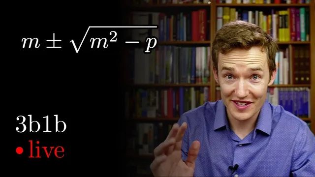
With that pattern in place, the quadratic formula is rebuilt for equations of the form ax²+bx+c=0. First, rescale so the leading coefficient becomes 1: divide by a to rewrite the quadratic as x² + b′x + c′. Next, use the fact that a monic quadratic with roots r and s factors as (x−r)(x−s). Expanding gives two key coefficient relationships: b′ equals the negative sum of the roots, and c′ equals the product of the roots. The remaining step is to express the roots as r,s = m ± d, where m is the midpoint (half the negative b′) and d is determined by the difference-of-squares identity: c′ = m² − d². Solving for d yields the “simpler quadratic formula” r,s = m ± √(m² − p), where p is the constant term after rescaling.
Practice examples show the method working on both real and complex cases. When the expression under the square root is negative, the roots become complex conjugates (e.g., 3 ± i), and the talk connects their magnitude to the constant term using the Pythagorean theorem in the complex plane. The episode closes by algebraically translating the simplified form back into the traditional quadratic formula, emphasizing that the “simpler” version is the same information, just routed through more interpretable intermediate structure.
Finally, the live stream ends with interactive polls about people’s relationship to the quadratic formula and playful “patronus” prompts, reinforcing the central theme: understanding patterns beats rote memorization.
Cornell Notes
The quadratic formula can be reconstructed without memorizing its full traditional form by using three structural facts about quadratics. After rescaling ax²+bx+c=0 into a monic quadratic x²+b′x+c′, the roots r and s satisfy (x−r)(x−s)=x²+b′x+c′, so b′=−(r+s) and c′=rs. Writing the roots as m±d turns the product rs into a difference of squares: (m−d)(m+d)=m²−d², letting d be found from d²=m²−c′. This yields r,s=m±√(m²−c′), and the same result matches the standard quadratic formula after algebraic simplification. The method also clarifies complex roots and links them to geometry in the complex plane.
Why does rescaling a quadratic (dividing by a) make the root-finding process easier?
How do the coefficients b′ and c′ determine the sum and product of the roots?
What role does the midpoint-and-distance representation r,s=m±d play?
How does the method handle quadratics with complex roots?
What is the “simpler quadratic formula” in the talk’s notation, and how is it equivalent to the standard one?
Review Questions
- Given a quadratic ax²+bx+c=0, what are the steps to compute its roots using the midpoint m and distance d method (including the rescaling)?
- For x²+b′x+c′=0, derive the relationship between b′, c′, and the roots r and s using (x−r)(x−s).
- If m²−c′<0 for a monic quadratic, what can be concluded about the roots, and how does the complex-plane interpretation fit that conclusion?
Key Points
- 1
Rescale ax²+bx+c=0 by dividing by a to get a monic quadratic x²+b′x+c′; this makes coefficient-to-root relationships immediate.
- 2
Use the factor form (x−r)(x−s)=x²−(r+s)x+rs to read off b′=−(r+s) and c′=rs.
- 3
Represent roots as r,s=m±d so the product becomes rs=m²−d², turning a product problem into a difference-of-squares problem.
- 4
Compute the midpoint as m=−b′/2 and then compute d from d²=m²−c′, giving roots m±√(m²−c′).
- 5
Complex roots arise naturally when m²−c′ is negative; the roots become conjugates and their magnitudes connect to the constant term via geometry in the complex plane.
- 6
The “simpler quadratic formula” is algebraically equivalent to the standard quadratic formula; it just routes through more interpretable intermediate structure.
- 7
The broader lesson is to treat algebraic identities (like difference of squares) as reusable patterns rather than isolated tricks.