This equation will change how you see the world (the logistic map)
Based on Veritasium's video on YouTube. If you like this content, support the original creators by watching, liking and subscribing to their content.
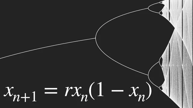
The logistic map X_{n+1} = R X_n (1 − X_n) produces extinction, steady states, oscillations, and chaos by changing only the growth-rate parameter R.
Briefing
A single, simple recurrence—known as the logistic map—can generate everything from stable population growth to sudden oscillations and full-blown chaos, and it does so in a way that matches real-world data across biology, physics, and even everyday dripping faucets. The key insight is that changing one parameter, the growth rate (often called R), doesn’t just shift outcomes smoothly; it triggers a cascade of “period-doubling” transitions. That cascade culminates in chaotic behavior where long-term prediction becomes effectively impossible, even though the underlying rule is deterministic.
The logistic map is written as X_{n+1} = R X_n (1 − X_n), where X represents the population as a fraction of a maximum possible limit (so X stays between 0 and 1). When R is small (below 1), the population declines toward extinction. Once R reaches 1, the system settles to a nonzero steady value. But as R increases further, the stable point breaks: the population starts bouncing between two values, then four, then eight, and so on. This “doubling of the period” is the hallmark of the route to chaos, and it mirrors what’s observed in nature—births and deaths (or other feedback processes) can produce repeating cycles that abruptly change as conditions shift.
At higher R values, the behavior becomes increasingly irregular. Around R ≈ 3.57, the system begins oscillating with longer repeating cycles; by R ≈ 3.83, stable periodic motion gives way to chaos. The striking part is that the chaotic regime isn’t random in a purely unstructured way: it contains windows of periodic stability, meaning order can reappear briefly inside the chaos. Zooming into the boundary between predictable and chaotic outcomes reveals a fractal structure.
That fractal structure connects directly to the Mandelbrot set. The branching diagram produced by the logistic map is essentially a slice of the Mandelbrot set, which is defined by iterating Z_{n+1} = Z_n^2 + C starting from Z_0 = 0. Values of C that keep the iterates bounded belong to the Mandelbrot set; those that blow up do not. The “Mandelbrot bulb” and its nested, self-similar features correspond to repeating periodic behaviors in the logistic map’s parameter space.
The same period-doubling pattern shows up in experiments and measurements beyond math. In fluid dynamics, temperature-driven convection in a mercury setup produced oscillations that halved and doubled in frequency as conditions changed. In neuroscience and animal behavior, eye-blink timing and cardiac arrhythmia in rabbits followed similar bifurcation sequences, and researchers used chaos theory to time electrical shocks to restore healthy rhythms. Even a dripping faucet can display period-doubling and chaotic dripping when the flow rate crosses certain thresholds.
Finally, the transcript highlights universality: the ratio between successive period-doubling intervals approaches the Feigenbaum constant (about 4.669). That constant appears across many different systems with different physical details, suggesting a deep, shared mathematical skeleton beneath complex behavior. The takeaway is less about rabbits or faucets and more about how simple deterministic rules can generate rich, structured unpredictability—and why that pattern keeps repeating across disciplines.
Cornell Notes
The logistic map X_{n+1} = R X_n (1 − X_n) models population growth with a built-in limit. For R < 1, the population declines to extinction; at R = 1 it settles to a fixed nonzero value. As R increases, the stable state breaks into oscillations that double their period repeatedly (2, 4, 8, …), producing a route to chaos. The boundary between stability and chaos forms a fractal pattern that connects to the Mandelbrot set, where bounded iteration defines membership. The same period-doubling behavior appears in real systems—from fluid convection and heart rhythms to dripping faucets—highlighting universality via the Feigenbaum constant (~4.669).
How does the logistic map decide between extinction, steady growth, and oscillations?
What is “period-doubling,” and why does it matter for predicting behavior?
Why does the logistic map’s parameter plot look fractal, and how does that connect to the Mandelbrot set?
What is the Feigenbaum constant, and what does its appearance imply?
How do real experiments mirror the logistic map’s bifurcation sequence?
Review Questions
- At what approximate values of R does the system transition from fixed-point stability to period-2 oscillations and then toward chaos, according to the transcript?
- Explain how bounded iteration in the Mandelbrot set definition relates to the appearance of stable periodic windows in the bifurcation diagram.
- Why does universality (including the Feigenbaum constant) suggest that chaos can emerge from many different kinds of systems?
Key Points
- 1
The logistic map X_{n+1} = R X_n (1 − X_n) produces extinction, steady states, oscillations, and chaos by changing only the growth-rate parameter R.
- 2
For R < 1, the population fraction X_n trends to 0; for R ≥ 1 it can settle to nonzero behavior before losing stability.
- 3
As R increases, the system undergoes a cascade of period-doubling transitions: 2-cycle, 4-cycle, 8-cycle, and so on.
- 4
The boundary between predictable and chaotic behavior forms a fractal structure that connects to the Mandelbrot set via boundedness of iterates.
- 5
Chaos is deterministic in rule but effectively unpredictable in practice because tiny differences in initial conditions can lead to diverging long-term outcomes.
- 6
Period-doubling and bifurcation patterns show up in real systems, including convection in fluids, heart rhythm dynamics, eye-blink timing, and dripping faucets.
- 7
The Feigenbaum constant (~4.669) captures a universal scaling law for how quickly period-doubling transitions accumulate across many different systems.