Transformer Circuits Part 1

Transformer circuits work centers on a simple but powerful claim: even in a stripped-down, one-layer attention-only Transformer, the model’s behavior can be decomposed into two interpretable “circuits”—an output value circuit that predicts how attending to a token changes the next-token logits, and a query-key circuit that predicts which tokens get attended to which others. That decomposition matters because it turns an opaque neural network into something closer to a set of mechanical rules: attention chooses sources, and learned linear maps decide how those sources shift the probability distribution over the vocabulary.

The discussion begins with a fast refresher on the Transformer architecture. Attention blocks (orange) sit alongside feed-forward networks (blue), and residual connections wrap both attention and feed-forward sublayers so that information flows forward even if learned weights are effectively zero. With stacked layers, the model repeatedly transforms a residual stream. For language modeling, tokens start as integer IDs (e.g., 0 to 49,999 for a 50,000-word vocabulary), get turned into vectors via an embedding matrix, and then produce a softmax over the vocabulary to predict the next token.

From there, the focus shifts to progressively simpler “toy” Transformers to make the math tractable. A “zero-layer Transformer” is treated as the simplest baseline: token IDs are embedded and then mapped through a product of embedding and unembedding matrices, yielding an approximation of bigram statistics. The key takeaway is that larger Transformers always contain a term with the same structure—an embedding-to-unembedding path—so understanding this baseline helps interpret what remains when attention is added.

The next step is the “one-layer attention-only Transformer,” which removes MLPs and simplifies away layer normalization and biases to reduce bookkeeping. At a high level, the model does three things: embed tokens, run each attention head and add its result into the residual stream, then map the final residual stream back to vocabulary logits via the unembedding matrix. Inside an attention head, the mechanism is described using matrices for values (from the residual stream via WV), attention weights (from queries and keys), and an output projection (WO) that decides how the attended information is written back into the residual stream.

A major conceptual move is to treat the full attention computation as a structured linear algebra object. By using tensor-product notation, the analysis separates “what attention moves” from “where it moves it.” In this framing, the query-key side determines an attention pattern across token positions (which token attends to which other token), while the value/output side determines how the attended token’s content changes the output logits. When the attention pattern is treated as fixed, the remaining computation becomes linear, allowing the model’s effect to be written as an identity term plus a sum of circuit terms.

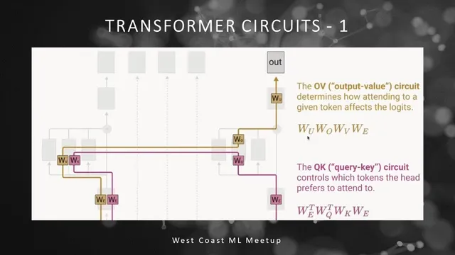
Two specific matrices become central. The output value circuit is effectively a vocabulary-by-vocabulary matrix formed from the embedding, value, output projection, and unembedding weights; it quantifies how attending to a particular token would bump or suppress specific vocabulary logits. The query-key circuit is another vocabulary-by-vocabulary matrix that yields pre-softmax attention affinities between token pairs, acting like a lookup table for which words are likely to attend to which others. The analysis notes that positions can matter in real models, but the simplified treatment initially ignores positional embeddings.

The session ends by emphasizing that this is a “lift the hood” approach: fully reverse-engineering a toy Transformer provides interpretability tools, even though multi-layer Transformers introduce more complex interactions. The next step is to test whether the predicted circuit behavior shows up in trained one-layer attention-only models and then extend the method to deeper architectures where interactions go beyond simple word-to-word affinity.