Why π is in the normal distribution (beyond integral tricks)

TL;DR

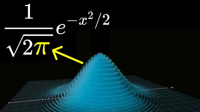
The area under the unnormalized bell curve e^(−x^2) equals √π, and dividing by √π makes the Gaussian integrate to 1.

Briefing Cornell Notes

Briefing

Pi’s appearance in the normal distribution isn’t a coincidence of algebra—it comes from geometry and from the way Gaussian shapes are forced by symmetry and independence. The normal (Gaussian) curve has the form proportional to e^(−x^2), and the constant that makes its total probability equal to 1 is tied to the integral of e^(−x^2). The key quantity is the area under the bell curve, which turns out to be √π; dividing by √π normalizes the distribution.

A classic proof gets √π by temporarily abandoning the “area under a curve” problem and instead computing the “volume under a bell surface” in three dimensions. Using the radially symmetric function e^(−r^2), where r is distance from the origin, the surface has circular symmetry around the z-axis. That symmetry allows the volume to be chopped into thin cylindrical shells: each shell contributes roughly (circumference)×(height)×(thickness). The circumference brings in a factor of 2πr, so π is pulled out naturally. The remaining integral becomes manageable because the integrand is set up so that the calculus antiderivative is available, yielding a total volume of π.

That three-dimensional volume then links back to the original two-dimensional area through a second slicing argument. If the same bell surface is sliced by planes parallel to the x-axis, each slice looks like the original one-dimensional bell curve e^(−x^2), just scaled vertically by a factor depending on the slice’s y-value. Because the function e^(−x^2−y^2) factors as e^(−x^2)·e^(−y^2), the slice areas are all proportional to one constant—exactly the unknown area under e^(−x^2). Integrating those slice areas across all y shows that the total volume equals (that unknown area)². Since the volume is already known to be π, the area under e^(−x^2) must be √π. That’s the direct route from π to the normalization constant in the Gaussian.

But the deeper question—why e^(−x^2) is special in statistics—gets answered by a 19th-century derivation due to John Herschel and later independently by James Clerk Maxwell. Start in two dimensions and demand two properties: (1) radial symmetry, meaning probability depends only on distance from the origin, not direction; and (2) independence of x and y, meaning the joint density factors into an x-part times a y-part. Those constraints force the radial dependence to satisfy a functional equation whose continuous solutions are exponential in r². After normalization, only the negative exponent works, producing the Gaussian shape e^(−const·r²). Maxwell’s three-dimensional statistical mechanics version reaches the same structure for molecular velocities.

Finally, the connection to the central limit theorem is the remaining bridge: in practice, normal distributions emerge from adding many independent variables, and the Gaussian is the unique stable shape consistent with that limiting behavior. The π-in-the-normal story therefore has two legs: geometry explains the √π normalization, while Herschel–Maxwell reasoning explains why the exponential of a squared distance is the natural form that independence and symmetry demand.

Cornell Notes

The Gaussian’s normalization constant is tied to π because the area under e^(−x^2) equals √π. A classic proof computes the volume under the radially symmetric surface e^(−r^2) in 3D, where cylindrical shells introduce a factor of π. Re-slicing the same volume into x-parallel slices shows that this 3D volume equals the square of the unknown 2D area under e^(−x^2), forcing that area to be √π. The transcript then explains why e^(−x^2) is not arbitrary: Herschel (and later Maxwell) derived the Gaussian from two requirements—radial symmetry and independence of coordinates—leading to an exponential in r² with a negative constant after normalization.

Why does computing a 3D “volume under a bell surface” help find the 2D area under e^(−x^2)?

Because the 3D surface e^(−r^2) is radially symmetric, its volume can be computed cleanly using cylindrical shells, which naturally introduce π via the shell circumference 2πr. Then the same volume can be computed again by slicing with planes parallel to an axis: each slice has the same bell-curve shape e^(−x^2), scaled by a factor depending on y. Since e^(−x^2−y^2) factors as e^(−x^2)·e^(−y^2), the slice areas are proportional to one constant—the unknown area under e^(−x^2). Integrating slice areas across all y makes the total volume equal to (that constant)². With the volume already found to be π, the constant must be √π.

What exact role does circular symmetry play in the appearance of π?

Circular symmetry makes the 3D integrand depend only on r, the distance from the origin, so points on the same circle share the same height e^(−r^2). When the volume is computed using cylindrical shells, each shell’s circumference is 2πr. That circumference factor is where π enters the calculation directly, before any normalization step for the 1D Gaussian.

Why can’t e^(−x^2) be integrated using elementary antiderivatives?

The transcript notes that an antiderivative exists but cannot be expressed using standard elementary functions (polynomials, trig functions, exponentials, and combinations). That’s why the proof uses a trick—moving to higher dimensions and using symmetry—to evaluate the definite integral indirectly.

How do Herschel’s two assumptions force the Gaussian form?

Herschel’s setup in 2D assumes (1) radial symmetry: the density depends only on distance r from the origin, not direction; and (2) coordinate independence: the joint density factors into an x-only part times a y-only part. Together, these imply a functional equation for the radial dependence that turns addition in the exponent into multiplication of function values. Under continuity, the only solutions are exponentials, giving a form e^(c·r²). Normalization requires c to be negative, yielding e^(−const·r²), i.e., the Gaussian shape.

Why does the constant in the exponent have to be negative?

If the exponent constant c were positive, e^(c·r²) would blow up as r→∞, making the total volume/probability infinite and preventing normalization. Only a negative constant makes the integral converge, allowing the distribution to be rescaled into a valid probability distribution.

How does Maxwell connect the same reasoning to real statistical mechanics?

Maxwell independently repeated the Herschel-style derivation in three dimensions while studying molecular velocities in a gas. The same structural requirements—symmetry and independence—again force an exponential in squared distance, producing the Gaussian distribution for velocity components. This makes the Gaussian feel less like a mathematical artifact and more like a consequence of physical assumptions.

Review Questions

In the 3D volume proof, how does the factorization e^(−x^2−y^2)=e^(−x^2)·e^(−y^2) enable the second slicing argument to relate the volume to the square of the 1D area?
What functional equation arises from Herschel’s radial symmetry plus coordinate independence, and why does continuity restrict its solutions to exponentials?
Why does normalization rule out positive constants in the exponent of the Gaussian form e^(c·r²)?

Key Points

1
The area under the unnormalized bell curve e^(−x^2) equals √π, and dividing by √π makes the Gaussian integrate to 1.
2
A classic derivation computes the 3D volume under e^(−r^2) using cylindrical shells, where the shell circumference contributes a factor of π.
3
Re-slicing the same 3D volume into axis-parallel slices shows the total volume equals the square of the 1D area under e^(−x^2).
4
Herschel’s derivation forces the Gaussian shape from two principles: radial symmetry (depends only on distance) and independence of coordinates (joint density factors).
5
The resulting functional equation has continuous solutions that are exponentials in r²; normalization requires the exponent constant to be negative.
6
Maxwell independently reached the same Gaussian structure in three dimensions while deriving velocity distributions in gases.
7
The central limit theorem provides the practical reason normal distributions emerge when many independent variables are added, tying the Gaussian’s form to limiting behavior.

Highlights

The √π normalization constant comes from geometry: the 3D volume under e^(−r^2) is π, and that volume equals the square of the 1D area under e^(−x^2).

π enters the proof not through algebraic manipulation but through circular symmetry: cylindrical shells contribute a circumference factor 2πr.

Herschel’s two assumptions—radial symmetry and coordinate independence—force the density to be exponential in r², leading directly to the Gaussian after normalization.

Maxwell’s independent derivation in statistical mechanics shows the same mathematical structure arises from physical modeling of molecular velocities.

Topics

Gaussian Normalization
Integral of e^(-x^2)
Herschel Maxwell Derivation
Radial Symmetry
Central Limit Theorem Connection

Mentioned

John Herschel
James Clerk Maxwell
Eugene Wigner
Kevin Ega