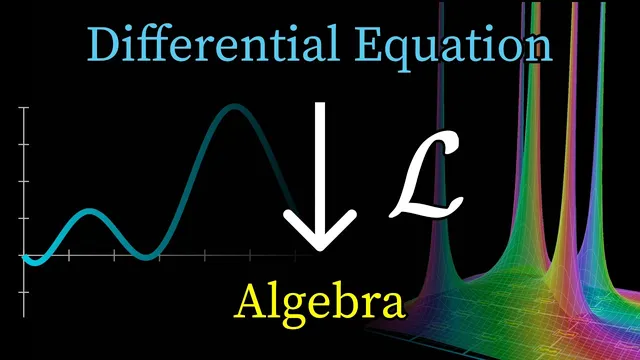
Why Laplace transforms are so useful

TL;DR

Laplace transforms convert time derivatives into multiplication by s in the transformed domain, with subtraction terms that encode initial position and velocity.

Briefing Cornell Notes

Briefing

A damped mass–spring system driven by a periodic external force settles into a steady oscillation at the *driving* frequency, while a second, transient motion tied to the system’s natural frequency fades away. The “wibbly startup” comes from two competing sets of terms in the solution: decaying modes from the unforced oscillator and a persistent cosine mode forced by the external wind. Laplace transforms make that split visible and computable by turning differential equations into algebra in the complex s-plane, where the locations of poles directly predict oscillation and decay.

The setup begins with a classic harmonic oscillator: a mass m attached to a spring with stiffness k, optionally damped by a term proportional to velocity with coefficient μ. Without forcing, the system oscillates at its natural frequency determined by the parameters, and damping makes those oscillations decay. Add a third force—an external oscillation modeled as a cosine—and the motion initially looks irregular: the amplitude swells and shrinks before locking into a regular rhythm. Laplace transforms provide a systematic way to analyze exactly why that transient phase lasts and what the eventual steady-state amplitude will be.

The key tool is the Laplace transform’s handling of derivatives. Taking the Laplace transform of f′(t) turns differentiation in time into multiplication by s in the transformed domain, but with a correction term that subtracts the initial value f(0). Applying the rule again shows that higher derivatives become higher powers of s, again with built-in initial-condition terms. This is the mechanism that converts the original differential equation into a rational expression: a polynomial in s multiplying the transformed unknown X(s), plus extra terms encoding initial position and velocity.

With the simplifying assumption that the mass starts from rest (x(0)=0 and x′(0)=0), the transformed equation yields a denominator that factors into two groups of poles. One group comes from the oscillator’s characteristic polynomial (the “mirror image” of the unforced dynamics). Those poles typically have negative real parts (so their contributions decay) and nonzero imaginary parts (so they oscillate). The other group comes from the Laplace transform of the forcing term cos(ωt), producing poles at s = iω and s = −iω. Those poles lie on the imaginary axis, meaning they generate a persistent oscillation with frequency ω and no decay.

In the s-plane picture, the transient “startup” corresponds to the decaying pole contributions still being significant early on; as time passes, those left-half-plane poles fade, leaving only the imaginary-axis poles. That’s why the system eventually follows a clean cosine synced to the external force, even when the driving frequency is unrelated to the spring’s natural resonant frequency.

To get an explicit time-domain formula, the rational expression in X(s) is decomposed into partial fractions. Each pole location becomes an exponential term in time, and pairs of complex-conjugate imaginary poles combine into a cosine for the steady state. The remaining algebra determines the amplitude, which depends on how close the driving frequency is to the resonant frequency—an insight with practical stakes for engineering structures like bridges.

Finally, the derivative-to-multiplication rule is justified in three ways: by checking it on exponentials (where differentiation is simple), by deriving it from the Laplace transform definition using integration by parts, and by connecting it to the deeper structure of inverse Laplace transforms—hinting at contour integrals and a unified theory that will be developed next.

Cornell Notes

Laplace transforms turn differential equations into algebra by mapping time derivatives to multiplication by s, with correction terms that automatically incorporate initial conditions. For a damped mass–spring system driven by a cosine force, the transformed solution X(s) has poles coming from two sources: the oscillator’s natural dynamics and the forcing frequency. Poles with negative real parts produce oscillations that decay, explaining the irregular startup phase. Poles at s = ±iω produce a non-decaying cosine at the driving frequency, explaining the eventual steady rhythm. Partial fraction decomposition then converts the pole structure back into an explicit time-domain solution, including the steady-state amplitude and its dependence on frequency mismatch.

Why does the mass–spring motion look irregular at first, then become a clean cosine?

The Laplace-domain solution splits into contributions from two pole sets. Poles tied to the unforced oscillator typically sit in the left half of the s-plane (negative real part), so their oscillations decay over time; they dominate early behavior and create the “wibbly” transient. Poles from the cosine forcing sit at s = iω and s = −iω on the imaginary axis, producing a persistent oscillation at frequency ω. As the decaying poles fade, the imaginary-axis poles remain, leaving only the steady cosine synced to the external force.

How does the Laplace transform convert differentiation into algebra, and where do initial conditions enter?

For a function f(t), the Laplace transform of its derivative satisfies L{f′(t)} = sF(s) − f(0). Applying the rule again gives L{f′′(t)} = s^2F(s) − s f(0) − f′(0). Those subtracted terms are exactly the initial position and initial velocity, so initial conditions are built into the transformed equation automatically rather than added later.

What do poles in X(s) tell you about oscillation and stability?

In the s-plane, the real part of a pole controls growth or decay: negative real parts correspond to decay, positive real parts to instability, and purely imaginary poles correspond to sustained oscillation. Imaginary parts correspond to oscillation frequency. In this driven oscillator, the unforced-system poles usually have negative real parts (decaying oscillations), while the forcing poles at ±iω lie on the imaginary axis (no decay), guaranteeing a steady response at the driving frequency.

Why does a cosine forcing term produce poles at s = ±iω?

The Laplace transform of cos(ωt) yields a rational function with denominator s^2 + ω^2. Setting s^2 + ω^2 = 0 gives s = iω and s = −iω. Those poles translate back into time-domain oscillations at frequency ω, matching the external forcing rhythm.

How does partial fraction decomposition produce the time-domain solution?

Once X(s) is written as a rational function, factoring the denominator reveals pole locations. The expression is decomposed into a sum of simpler fractions whose denominators look like (s − s_k). Inverting each term uses the rule that fractions of that form correspond to exponentials e^{s_k t}. Complex-conjugate imaginary poles combine into cosines, giving the steady-state oscillation, while left-half-plane poles contribute decaying exponentials.

What frequency relationship matters for the steady-state amplitude?

The steady-state amplitude depends on how close the driving frequency ω is to the system’s resonant frequency determined by m, μ, and k (through the roots of the oscillator’s characteristic polynomial). As ω approaches resonance, the amplitude grows; as the mismatch increases, the steady response weakens. This is the same principle behind avoiding destructive wobble in structures like bridges.

Review Questions

In the Laplace-domain solution for a driven damped oscillator, which pole locations correspond to transient decay versus persistent oscillation, and how can you tell from their positions in the s-plane?
How do the terms involving f(0) and f′(0) arise when transforming second derivatives, and why are they essential for matching the initial physical state?
If the external force were not cos(ωt) but another periodic function, what would you expect to change in the pole structure of X(s), and how would that affect the long-term motion?

Key Points

1
Laplace transforms convert time derivatives into multiplication by s in the transformed domain, with subtraction terms that encode initial position and velocity.
2
For a damped mass–spring system driven by cos(ωt), the transformed solution has poles from both the natural oscillator dynamics and the forcing term.
3
Poles with negative real parts generate oscillations that decay, explaining the irregular startup before steady behavior emerges.
4
Poles at s = ±iω generate a persistent cosine at the driving frequency, explaining why the long-term motion locks to the external rhythm.
5
The “wibbly startup” is the period when decaying natural-mode contributions are still significant compared with the non-decaying forced-mode contribution.
6
Partial fraction decomposition maps pole locations back into exponentials in time, and complex-conjugate imaginary poles combine into cosines.
7
The steady-state amplitude depends strongly on the frequency mismatch between the driving frequency and the system’s resonant frequency, with direct engineering implications.

Highlights

The transient phase comes from left-half-plane poles (decaying oscillations), while the eventual steady rhythm comes from imaginary-axis poles at s = ±iω.

Differentiation becomes algebra: L{f′(t)} = sF(s) − f(0), so initial conditions are automatically incorporated in the transformed equation.

A cosine forcing term produces a denominator s^2 + ω^2, guaranteeing poles at s = iω and s = −iω and thus a long-term response at frequency ω.

Partial fractions turn pole structure into explicit time-domain terms; pole locations become exponents, and conjugate imaginary poles combine into cosines.

Resonance is not just a qualitative idea here: the amplitude of the steady-state cosine depends on how close ω is to the natural resonant frequency set by m, μ, and k.

Topics

Laplace Transforms
Driven Oscillations
s-Plane Poles
Initial Conditions
Partial Fractions