Why “probability of 0” does not mean “impossible” | Probabilities of probabilities, part 2

TL;DR

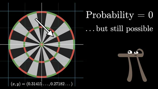
In continuous probability, exact point probabilities like P(h = 0.7) are 0, even though the parameter still has total probability 1 across all values.

Briefing Cornell Notes

Briefing

Assigning a nonzero probability to every exact real value of an unknown parameter leads to a paradox: there are uncountably many candidate values, so either the total probability “blows up” if each point gets some positive weight, or it collapses to zero if each point gets probability 0. The fix is to stop treating individual real numbers as the basic units of probability and instead treat intervals (ranges) as the fundamental objects.

The setup begins with a weighted coin whose true probability of heads is an unknown number h between 0 and 1. After observing 10 tosses with 7 heads, the natural question becomes: what is the probability that h equals 0.7? Phrased that way, the question is “probability of a probability,” and it also demands an answer about a single point in a continuum. In a continuous setting, any specific exact value like h = 0.7 has probability 0, even though the overall parameter h still has total probability 1 across all possibilities. If one tries to assign nonzero probability to each exact value, the sum over infinitely many points cannot remain finite.

The resolution comes from coarse-graining: group possible values of h into buckets, such as 0.80–0.85, and ask for the probability that h falls inside each bucket. Crucially, the probability is represented by the area of each bar, not its height. As buckets get narrower, the probability of landing in any single tiny interval shrinks toward 0, but the bar’s height approaches a stable “density” level because the interval width is shrinking. In the limit, the collection of bars becomes a smooth curve: the probability density function (PDF).

This reframes what the vertical axis means. The height is not a probability; it is probability per unit length along the h-axis. The total probability remains 1 because the total area under the curve across [0, 1] stays fixed. Under this rule, the probability that h lies between two values a and b is the area under the PDF between a and b. A single point corresponds to an interval of width 0, so its probability is 0, while the probabilities of all intervals together still sum to 1.

The shift is not just a visualization trick; it reflects a change in the underlying “rules” for continuous probability. In discrete cases, probabilities of individual outcomes can be added. In continuous cases, probabilities of ranges are the primitive quantities, and individual points are treated as degenerate ranges. Measure theory provides the rigorous framework that unifies these discrete and continuous viewpoints by defining how probability assignments behave across sets.

With that foundation in place, the original coin question becomes well-posed: after observing tosses, the goal is to find the PDF for h. Once that density is known, it becomes straightforward to answer questions like the probability that the true heads probability lies between 0.6 and 0.8. The next step is to compute that posterior density from the observed data.

Cornell Notes

The paradox of “probability of 0” comes from trying to assign probability to exact real values of an unknown parameter h. In a continuum, each exact value (like h = 0.7) has probability 0, yet the parameter still has total probability 1 across all possibilities. The cure is to treat intervals as the basic units: build buckets for h, and represent probability by bar area (width × height). As buckets get finer, the bars’ heights converge to a probability density function (PDF), where probabilities for ranges equal the area under the curve. This makes statements about h precise—e.g., P(0.6 ≤ h ≤ 0.8) is an area—while point probabilities remain 0.

Why does asking for P(h = 0.7) create a paradox in continuous settings?

Because h can take uncountably many exact real values in [0, 1]. If every exact value were assigned a nonzero probability, adding them all would not stay finite. If instead each exact value gets probability 0, then summing over points gives 0, even though the total probability over all h must be 1. The paradox signals that point probabilities are not the right primitive objects in a continuum.

How does “probability as area” resolve the issue?

When h is binned into intervals (e.g., 0.80–0.85), the probability of landing in that interval is represented by the area of the corresponding bar. As intervals get narrower, the probability of any single bucket shrinks, but the bar height approaches a stable value (the density). In the limit, the curve’s area over any range gives the probability for that range, while a single point corresponds to zero-width area and thus probability 0.

What does the height of a PDF mean if it’s not a probability?

The height is probability density: probability per unit length along the h-axis. That’s why probability for an interval [a, b] is computed as the area under the PDF between a and b, not by reading the height at a point. This keeps the total probability equal to 1 because the total area under the curve across [0, 1] is 1.

How do continuous probability rules differ from discrete ones?

In discrete settings, probabilities of individual outcomes can be added. In continuous settings, probabilities of ranges are fundamental, and individual points are treated as degenerate intervals of width 0. So the meaningful probability statements are about intervals, not exact values.

What role does measure theory play in making this rigorous?

Measure theory supplies an axiom system that defines how to assign numbers like probabilities to sets (including intervals) in a way that behaves consistently across both discrete and continuous cases. It formalizes the intuition that sums over points in discrete cases become integrals over ranges in continuous cases.

After observing coin tosses, what is the correct target object to compute?

The probability density function (PDF) for the unknown heads probability h after updating on the observed data. Once the PDF is known, questions about h become area calculations—such as the probability that h lies between 0.6 and 0.8.

Review Questions

In a continuum, why must probabilities of exact values be treated differently from probabilities of intervals?
Explain why representing probability by bar height fails as buckets get infinitely thin, and why representing probability by bar area succeeds.
Given a PDF for h on [0, 1], how would you compute P(0.6 ≤ h ≤ 0.8) and why is P(h = 0.7) equal to 0?

Key Points

1
In continuous probability, exact point probabilities like P(h = 0.7) are 0, even though the parameter still has total probability 1 across all values.
2
The basic units of probability in a continuum are intervals (ranges), not individual real numbers.
3
Represent probability for a range by the area under a curve; the PDF’s height is density, not probability.
4
As bins get narrower, bucket probabilities shrink but density heights stabilize, producing a smooth PDF in the limit.
5
Probability for a range [a, b] equals the area under the PDF between a and b; a single point has zero-width area.
6
Discrete “sum of probabilities” logic changes to continuous “integral of densities” logic because the underlying rule system is different.
7
Measure theory provides the rigorous framework that unifies discrete and continuous probability assignments.

Highlights

Trying to assign nonzero probability to every exact real value of h leads to an infinite total; assigning zero to each point makes the total collapse—both outcomes reveal the wrong unit of probability.

Using bar area (width × height) turns the paradox into a coherent picture: bucket probabilities become areas, and the curve’s total area stays 1.

A PDF’s value at a point is not a probability; only the area over an interval corresponds to probability.

In continuous settings, probabilities of ranges are primitive, while probabilities of individual points are treated as degenerate intervals of width 0.

Once the posterior PDF for the unknown coin bias h is found, questions like P(0.6 ≤ h ≤ 0.8) become straightforward area computations.

Topics

Probability Density Functions
Continuous Probability
Probability of Probability
Measure Theory
Bayesian Updating