A Comprehensive Tutorial on Correlation Analysis using SPSS Combined

Q: How should R be interpreted in terms of direction and strength?

R ranges from -1 to +1. A positive R means the variables move together: as one increases, the other tends to increase. A negative R means an inverse relationship: as one increases, the other tends to decrease. Strength is read from the magnitude of R using practical guidelines: |R| ≤ 0.1 very weak, 0.1–0.3 weak, 0.3–0.5 moderate, 0.5–0.7 strong, and >0.7 very strong. The tutorial also warns that extremely high correlations (around 0.85+) may indicate multi-collinearity, meaning the constructs are nearly identical.

Q: What does p < 0.05 mean in correlation analysis, and how does it connect to hypotheses?

The tutorial uses the common social-science rule: if the p-value is less than 0.05, the relationship is considered statistically significant. In hypothesis terms, this leads to rejecting the null hypothesis of no association and accepting the alternate hypothesis that a relationship exists. In the example, the correlation between “vision” and “organizational performance” is significant because the p-value is below 0.05.

Q: How do you handle correlation analysis when there are more than two variables?

Instead of running separate pairwise correlations, the tutorial uses SPSS’s correlation matrix by adding a third (and additional) variable(s) in “Analyze → Correlate → Bivariate.” The output becomes a matrix showing Pearson correlations between every pair. Researchers can select one-tailed tests when theory predicts a specific direction (positive or negative) and two-tailed tests when direction is uncertain. For reporting, the matrix is formatted into a publication-ready table, often removing redundant cells and reporting only significant or important correlations.

Q: What is the purpose of confidence intervals in correlation output?

Confidence intervals provide a range likely to contain the true population correlation. Because the true population parameter can’t be measured directly, bootstrapping generates lower and upper bounds (e.g., a 95% interval). The tutorial interprets this as: with 95% confidence, the true correlation lies between the reported lower and upper limits. This complements the point estimate of R and helps communicate uncertainty.

Q: How can correlations be compared across two groups, and what does “insignificant difference” imply?

The tutorial splits the dataset by group (e.g., gender) using “Data → Split File,” computes correlations within each subgroup, then tests whether the correlation coefficients differ significantly. It uses a “significance of difference between two correlations” calculator (Daniel Steiger’s method referenced). If the resulting p-value is greater than 0.05, the difference is treated as statistically insignificant—meaning the relationship strength appears effectively the same across groups.

TL;DR

Pearson correlation coefficient (R) quantifies the direction (sign) and strength (magnitude) of a linear relationship between two quantitative variables.

Briefing Cornell Notes

Briefing

Correlation analysis in SPSS hinges on one core statistic: the Pearson correlation coefficient (R), which quantifies both the direction and strength of a linear relationship between two quantitative variables. A positive R means higher values in one variable tend to align with higher values in the other; a negative R means the opposite. Because scatter plots can suggest patterns but can’t reliably measure strength, R provides the numerical yardstick—while significance testing (via p-values) determines whether the observed relationship is likely to reflect a real association rather than sampling noise.

Interpretation starts with practical guidelines for R’s magnitude. Values near 0 indicate very weak relationships, while values closer to 1 (or -1) indicate stronger linear association. The tutorial lays out a commonly used scale: |R| ≤ 0.1 is very weak, 0.1–0.3 weak, 0.3–0.5 moderate, 0.5–0.7 strong, and above 0.7 very strong. It also flags a key caution: very high correlations (around 0.85 or more) can signal multi-collinearity—when two constructs are essentially measuring the same underlying concept.

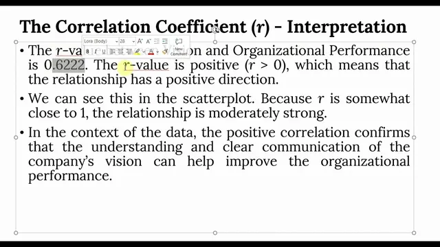
A worked example demonstrates how to run Pearson correlations in SPSS. Using composite variables (computed as means of multiple items) for “vision” and “organizational performance,” the output reports an R value (shown as 0.622 in the narrative) and a p-value below the 0.05 threshold, leading to the conclusion that the relationship is statistically significant. The tutorial emphasizes that significance is assessed first (p < 0.05 in social science research), and then strength is interpreted using the R magnitude. It also notes that correlation alone doesn’t confirm linearity: researchers should pair R with a scatter plot and check whether points cluster around a fitted line. In the example, the scatter plot shows an upward tendency consistent with a positive linear relationship.

For reporting, the tutorial distinguishes between bivariate correlation and multi-variable correlation matrices. With more than two variables, SPSS produces a matrix of Pearson correlations, and researchers can choose one-tailed or two-tailed significance depending on whether the direction of the relationship is theoretically expected. The results are then formatted into a clean table for publication, typically removing redundant cells and reporting only meaningful correlations. When confidence intervals are needed, SPSS’s correlation procedure with confidence intervals uses bootstrapping (with 1,000 samples by default in the walkthrough) to produce lower and upper bounds around the correlation estimate—allowing researchers to state a plausible range for the true population correlation (e.g., a 95% interval).

Finally, the tutorial addresses comparing correlations across groups. It shows how to split the dataset by gender, compute correlations separately for male and female, and then test whether the difference between two correlation coefficients is statistically significant. Using a “significance of difference between two correlations” calculator (Daniel Steiger’s method referenced), the example finds that the male vs. female difference is insignificant (p > 0.05), implying the strength of the relationship between organizational commitment and collaborative culture is effectively the same across genders.

Cornell Notes

Pearson correlation coefficient (R) measures the direction and strength of a linear relationship between two quantitative variables. The sign of R indicates direction (positive vs. negative), while the magnitude indicates strength, using common cutoffs such as very weak (≤0.1), weak (0.1–0.3), moderate (0.3–0.5), strong (0.5–0.7), and very strong (>0.7). Statistical significance is judged using p-values (typically p < 0.05 in social science research), and linearity should be checked with a scatter plot and fitted line because R alone doesn’t confirm linear form. For multiple variables, SPSS outputs a correlation matrix; for uncertainty, confidence intervals via bootstrapping provide lower and upper bounds for the true population correlation. Correlations can also be compared across groups by splitting data and testing whether the difference between correlation coefficients is significant.

How should R be interpreted in terms of direction and strength?

R ranges from -1 to +1. A positive R means the variables move together: as one increases, the other tends to increase. A negative R means an inverse relationship: as one increases, the other tends to decrease. Strength is read from the magnitude of R using practical guidelines: |R| ≤ 0.1 very weak, 0.1–0.3 weak, 0.3–0.5 moderate, 0.5–0.7 strong, and >0.7 very strong. The tutorial also warns that extremely high correlations (around 0.85+) may indicate multi-collinearity, meaning the constructs are nearly identical.

Why isn’t a significant correlation enough to claim a linear relationship?

Correlation coefficient measures strength of linear association, but it doesn’t prove the relationship is linear. The tutorial pairs R with a scatter plot and a fitted line (e.g., “fit line total” in SPSS). If points cluster closely around the line, linearity is more credible; if points curve or scatter widely, the relationship may not be linear even if R is non-zero.

What does p < 0.05 mean in correlation analysis, and how does it connect to hypotheses?

The tutorial uses the common social-science rule: if the p-value is less than 0.05, the relationship is considered statistically significant. In hypothesis terms, this leads to rejecting the null hypothesis of no association and accepting the alternate hypothesis that a relationship exists. In the example, the correlation between “vision” and “organizational performance” is significant because the p-value is below 0.05.

How do you handle correlation analysis when there are more than two variables?

Instead of running separate pairwise correlations, the tutorial uses SPSS’s correlation matrix by adding a third (and additional) variable(s) in “Analyze → Correlate → Bivariate.” The output becomes a matrix showing Pearson correlations between every pair. Researchers can select one-tailed tests when theory predicts a specific direction (positive or negative) and two-tailed tests when direction is uncertain. For reporting, the matrix is formatted into a publication-ready table, often removing redundant cells and reporting only significant or important correlations.

What is the purpose of confidence intervals in correlation output?

Confidence intervals provide a range likely to contain the true population correlation. Because the true population parameter can’t be measured directly, bootstrapping generates lower and upper bounds (e.g., a 95% interval). The tutorial interprets this as: with 95% confidence, the true correlation lies between the reported lower and upper limits. This complements the point estimate of R and helps communicate uncertainty.

How can correlations be compared across two groups, and what does “insignificant difference” imply?