A pretty reason why Gaussian + Gaussian = Gaussian

TL;DR

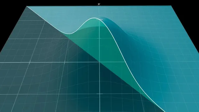
Convolution at s can be interpreted as the integrated probability density over the diagonal slice x+y=s for independent variables.

Briefing Cornell Notes

Briefing

Adding two independent normally distributed variables produces another normal distribution—a “stability” result that explains why the Gaussian is the central shape behind the central limit theorem. The key computation is the convolution of two Gaussian functions, and the payoff is that the convolution’s output keeps the same functional form, with the spread increasing in a predictable way.

The starting point is the simplified bell-curve kernel e^{-x^2}. Convolution asks how likely it is that two independent samples (one drawn from each Gaussian) land on pairs (x, y) whose sum x + y equals a target value s. Geometrically, that probability comes from integrating the product e^{-x^2}e^{-y^2} over the “diagonal slice” of the xy-plane defined by x + y = s. For generic functions, those slices create messy shapes and the integral offers little intuition. Gaussian functions are different: the product e^{-x^2}e^{-y^2} depends only on x^2 + y^2, the squared distance from the origin, which makes the entire 3D surface rotationally symmetric.

That symmetry is the engine of the shortcut. Because the slice x + y = s sits at a fixed perpendicular distance from the origin—specifically s/√2—the diagonal slice area matches the area of a rotated slice. Rotating by 45 degrees turns the problem into one where the slice is parallel to an axis, so one variable becomes constant along the slice. The remaining integral then separates cleanly into an s-dependent exponential factor and an s-independent constant. The s-dependent part becomes e^{-s^2/2}, showing that the convolution has the same bell-curve shape as a Gaussian, just with a different width. The leftover constant is √π (and a technical normalization factor of 1/√2 adjusts the exact convolution value), but the structural conclusion is what matters: convolving two Gaussians yields another Gaussian.

Restoring the full normal-distribution parameters (mean 0 and standard deviation σ) leads to the standard result: the sum of two independent N(0, σ^2) variables is distributed as N(0, (√2 σ)^2). In other words, the standard deviation scales by √2. This is special because most convolution operations do not preserve the original family of functions; they typically produce entirely new shapes.

That specialness also clarifies the central limit theorem’s “why.” The theorem says repeated addition of independent finite-variance random variables tends toward a universal limiting distribution after shifting and rescaling. But the Gaussian’s role isn’t a coincidence or a consequence of the theorem alone: the convolution calculation shows that Gaussians are fixed points under the repeated-convolution process. In a common proof strategy, one first shows convergence to some universal shape for a broad class of starting distributions, then uses the fact that Gaussian-to-Gaussian convolution leaves the Gaussian unchanged to identify that universal limit as the Gaussian itself. The same rotational-symmetry geometry also connects to other derivations of the bell curve and to classic appearances of π, tying the geometry of x^2 + y^2 directly to the central limit phenomenon.

Cornell Notes

Convolution measures how the sum of two independent random variables distributes. For Gaussian kernels e^{-x^2}, the product e^{-x^2}e^{-y^2} depends only on x^2+y^2, giving rotational symmetry in the xy-plane. That symmetry lets diagonal slices x+y=s be treated as rotated, axis-parallel slices at distance s/√2 from the origin, separating the integral into an s-dependent factor and an s-independent constant. The s-dependent factor becomes e^{-s^2/2}, so the convolution of two Gaussians is another Gaussian. With standard deviation σ, the result is that adding two independent N(0,σ^2) variables yields N(0,2σ^2), i.e., standard deviation √2·σ—making Gaussians stable under the convolution step behind the central limit theorem.

Why does the convolution of two Gaussians stay Gaussian instead of turning into a new function?

Because the Gaussian product e^{-x^2}e^{-y^2}=e^{-(x^2+y^2)} depends only on x^2+y^2, the squared distance from the origin. That creates rotational symmetry in the 3D surface over (x,y). When computing the convolution at s, the relevant “diagonal slice” x+y=s has a fixed distance s/√2 from the origin, so the slice’s area matches an easier rotated slice. The integral then factors into an s-dependent exponential e^{-s^2/2} times an s-independent constant, leaving the Gaussian form intact.

How does the geometry of the line x+y=s lead to the exponent e^{-s^2/2}?

The line x+y=s intersects the axes at (s,0) and (0,s). The perpendicular distance from the origin to this line is s/√2 (a Pythagorean-geometry result). Rotational symmetry means the slice area depends only on that distance, not on the slice’s orientation. After rotating by 45 degrees, one coordinate becomes constant along an axis-parallel slice, so the remaining integral contributes only a constant while the distance term produces the exponent e^{-s^2/2}.

What role does the constant √π play, and why is it less important than the shape?

When the rotated slice reduces the problem to an integral over y with x fixed, the remaining integral is a classic one whose value is √π. There’s also a technical normalization factor (convolution value equals slice area divided by √2). These constants affect the overall scaling so the distribution integrates correctly, but the decisive feature is that the s-dependence becomes e^{-s^2/2}, proving the output is Gaussian in s.

How does the result change when the Gaussians have standard deviation σ instead of the simplified e^{-x^2} form?

Using the full normal form with mean 0 and standard deviation σ introduces σ into the exponent and normalization. The same “square-distance” and symmetry argument repeats, producing the same √2 factor in the exponent and in the width. The convolution corresponds to adding independent N(0,σ^2) variables, yielding N(0,2σ^2). Equivalently, the standard deviation becomes √2·σ.

How does this convolution fact connect to the central limit theorem’s proof strategy?

A common approach has two steps: first, show that repeated addition (repeated convolution with appropriate shifting/rescaling) converges to a single universal limiting distribution for many finite-variance starting distributions. That step doesn’t identify the limit. Second, identify the fixed point: convolving two Gaussians gives another Gaussian with a predictable rescaling, so Gaussians are stable under the convolution operation. Since the universal limit must be the only fixed point in that family, the limit is the Gaussian.

Why is rotational symmetry described as a “uniquely characterizing” feature of bell curves?

For the Gaussian, the exponent combines into x^2+y^2, so the surface depends only on distance from the origin. For most other symmetric smooth functions, the product of two copies does not collapse to a function of x^2+y^2 alone, so diagonal slices become complicated and the symmetry-based shortcut fails. That’s why the geometric intuition works cleanly for Gaussians but not generally for other distributions.

Review Questions

If the convolution at s is computed via integrating over the slice x+y=s, what geometric quantity determines the slice’s distance from the origin for the Gaussian case?
What property of e^{-(x^2+y^2)} enables the rotation argument, and how does that simplify the integral?
In the central limit theorem proof outline, why does showing Gaussian-to-Gaussian convolution act like a fixed point help identify the universal limiting distribution?

Key Points

1
Convolution at s can be interpreted as the integrated probability density over the diagonal slice x+y=s for independent variables.
2
For Gaussian kernels, the product depends only on x^2+y^2, creating rotational symmetry that makes diagonal slices equivalent to rotated axis-parallel slices.
3
The distance from the origin to the line x+y=s is s/√2, which drives the s-dependent exponential term e^{-s^2/2}.
4
The convolution of two Gaussians is another Gaussian: adding independent N(0,σ^2) variables yields N(0,2σ^2), so the standard deviation becomes √2·σ.
5
Gaussian stability under convolution explains why the Gaussian is the fixed point that the central limit theorem converges toward after rescaling.
6
A typical central limit theorem proof strategy uses a universal convergence step (existence of a single limit shape) plus the fixed-point property of Gaussians to identify that limit.
7
The same rotational-symmetry geometry links the Gaussian’s form to other derivations and to the appearance of π through a classic integral.

Highlights

Rotational symmetry turns a hard diagonal-slice convolution into an easier axis-parallel slice, separating the integral into an s-dependent Gaussian factor and an s-independent constant.

The line x+y=s sits at distance s/√2 from the origin; that single geometric number controls the exponent in the resulting convolution.

Convolving two Gaussians preserves the Gaussian family: standard deviation scales by √2 when adding independent normals.

The Gaussian’s “fixed point” behavior under convolution is the structural reason it emerges as the central limit theorem’s universal shape.

The √π constant comes from a classic integral, but the decisive result is the preserved e^{-s^2/2} dependence.

Topics

Convolution
Gaussian Distributions
Central Limit Theorem
Rotational Symmetry
Probability Geometry