Binary Logistic Regression Analysis using SmartPLS: How to Run, and Interpret the Results.

Binary logistic regression in SmartPLS4 can be run as a straightforward “plain regression” model to predict a binary outcome—here, whether respondents choose private versus public sector banks—using a set of predictor variables such as value-added services, perceived cost, and perceived risk. The workflow starts with importing the dataset, creating a new project, defining the dependent variable (Choice) and coding categories so that private bank choice is coded as 1 and public bank choice as 0. After placing the dependent variable and all predictors onto the model canvas, the model is calculated using default settings, producing coefficients, model-fit statistics, classification (confusion) metrics, and significance tests for each predictor.

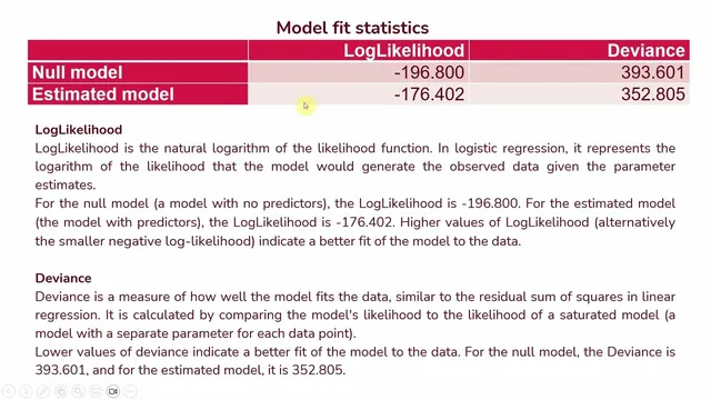
Interpretation hinges on three layers of output. First, model fit statistics determine whether the predictor-based model improves over a null model with no predictors. Log likelihood and deviance are compared between the null model and the estimated model: higher log likelihood (or, equivalently, a less negative log likelihood) and lower deviance indicate better fit. The session also emphasizes pseudo R-square—specifically NealK r²—as an approximate measure of how much variation in the criterion variable is captured by the predictors. In the example, NealK r² is 0.165, which is translated into an estimated 16.5% change in the criterion variable attributable to the predictors.

Second, information criteria such as AIC and BIC help balance fit against complexity. Lower AIC suggests a better trade-off between model accuracy and overfitting risk, while BIC penalizes complexity more heavily. The reported pattern is that AIC improves from the null model to the estimated model (dropping from 39561 to 37480.5), supporting the idea that the predictors add meaningful explanatory power without excessive cost in complexity. The session also notes that BIC can be higher when many predictors are included, even if other fit measures look good.

Third, classification performance is evaluated using confusion metrics. The model correctly predicts 61 cases when the observed outcome is 0 and correctly predicts 159 cases when the observed outcome is 1. Overall, it gets 64.5% of cases correct, computed as (61 + 159) divided by the total sample size. This “percentage accuracy” is presented as the practical measure of how well the model assigns respondents to the correct bank-choice category.

Finally, the coefficients determine which predictors matter and in what direction. Significance is assessed using p-values (derived from t or z statistics). Odds ratios translate coefficient effects into interpretable changes in the odds of choosing a private bank. An odds ratio greater than 1 means the predictor increases the likelihood of the target event (private bank choice); an odds ratio less than 1 means it decreases that likelihood. In the example, value-added services has an odds ratio of 1.373 and is significant, implying the odds of choosing a private bank are 1.373 times higher when value-added services are present. Perceived cost (odds ratio 0.782, significant) and perceived risk (odds ratio 0.601, significant) both fall below 1, indicating higher perceived cost or risk reduces the odds of choosing private banks relative to public banks.

Taken together, the approach provides a complete decision pipeline: verify model fit, check predictive accuracy, then interpret significant predictors through odds ratios to understand how each factor shifts the probability of private versus public bank choice.