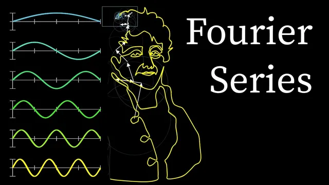
But what is a Fourier series? From heat flow to drawing with circles | DE4

Fourier series turn a messy, real-world initial condition—like a discontinuous step in temperature—into a controlled sum of simple, rotating components. The payoff is practical and conceptual: once a function is decomposed into frequency components, linear dynamics such as the heat equation become predictable because each frequency evolves independently, typically decaying at a rate tied to its frequency. That independence is what lets a swarm of rotating arrows trace out a target shape over time, and it’s why Fourier’s idea became foundational far beyond heat.

The story begins with the heat equation on a rod. When the initial temperature profile is a cosine wave tuned to satisfy boundary conditions, the solution is easy: the wave’s amplitude shrinks exponentially as time passes, and higher-frequency waves decay faster than lower-frequency ones. Linearity is the key structural property—solutions can be added and scaled—so any initial condition that can be written as a sum of such cosine waves can be evolved by evolving each wave separately. As time goes on, the faster-decaying high-frequency terms fade, leaving a smoother, low-frequency shape. In other words, the heat equation’s smoothing effect is encoded in the different decay rates of the frequency components.

That raises the central challenge Fourier tackled: most realistic initial conditions don’t look like tidy sine or cosine waves. A classic example is two rods brought into contact at opposite temperatures, producing a step function: flat at 1 on one side, flat at −1 on the other, with a jump discontinuity. Despite the step’s obvious mismatch with smooth oscillations, Fourier showed it can be represented as an infinite series of sine/cosine terms (subject to boundary conditions). For the step function, the coefficients follow a pattern involving odd frequencies—1, −1/3, 1/5, −1/7, and so on—scaled by 4/π. The representation is exact only in the infinite-sum sense: partial sums never perfectly match the discontinuity, but the limit does, with a subtle convention at the jump point.

To make the computations cleaner and to set up later tools, the discussion generalizes from real-valued functions to complex-valued functions that can be viewed as drawings in the complex plane. In this broader picture, each “frequency component” becomes a rotating vector on the unit circle. The fundamental building block is the complex exponential e^{i t}, which traces circles as t increases. A general Fourier decomposition expresses an arbitrary function f(t) (for t in [0,1]) as an infinite sum of terms c_n e^{2π i n t}, where the complex coefficients c_n determine the initial magnitudes and angles of each rotating vector.

Finding each coefficient becomes a clever filtering operation. The constant term c_0 is obtained by averaging f(t) over the interval, because every rotating non-constant term completes whole cycles and averages to zero. To extract c_n for any integer n, f(t) is multiplied by e^{−2π i n t} before averaging; this “freezes” the nth component while forcing all others to rotate through full cycles, again averaging them away. The resulting integral formula is the engine behind the animations: given a path (often imported from an SVG), the computer numerically approximates these integrals for a finite range of n, then reconstructs the drawing by summing the corresponding rotating vectors. As the number of vectors increases, the approximation converges toward the original path.

The heat-equation example and the rotating-vector framework converge on one larger lesson: exponential functions—especially complex exponentials—are the natural language for solving linear differential equations. Fourier series are not just a trick for oscillations; they’re a systematic way to break complicated behavior into components that evolve predictably under linear dynamics.