But what is a partial differential equation?

TL;DR

Model temperature as a function T(x, t) so every position has its own value that evolves over time.

Briefing Cornell Notes

Briefing

The heat equation turns the everyday idea of heat flowing from warm to cool into a precise rule for how an entire temperature profile evolves over time. Instead of tracking a handful of numbers, it treats temperature as a function of position and time—so every point along a rod has its own value—and then links the time-change of that function to how it curves in space. The payoff is big: this one equation becomes a template for diffusion phenomena across math and physics, from Brownian motion to finance’s black-Scholes model.

The setup begins with a rod along the x-axis, where temperature is written as T(x, t). Visualizing T as a surface over the x–t plane helps clarify why partial differential equations are different from ordinary ones: there are multiple independent directions in which change can occur. One derivative measures how temperature varies as you move along the rod (∂T/∂x), while another measures how temperature at a fixed location changes as time passes (∂T/∂t). Because both kinds of change matter at once, the heat equation uses partial derivatives—derivatives with respect to one variable while holding the others fixed.

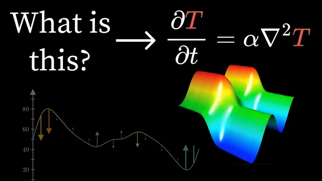
At the heart of the heat equation is a proportionality: the rate at which temperature changes in time is proportional to the second spatial derivative, ∂T/∂t = α ∂²T/∂x² (with α as a constant). Intuitively, the second derivative captures curvature. Where the temperature profile bends upward, the “slope of the slope” is positive, and temperature tends to rise; where it bends downward, that curvature is negative and temperature tends to fall. In plain terms, curved regions flatten out over time, because each point is pulled toward the average behavior of its neighbors.

That neighbor-averaging intuition is derived by first discretizing the rod into finitely many points. For a point T2 flanked by T1 and T3, the tendency of T2 to heat or cool depends on whether the average of its neighbors is above or below it. Rewriting the neighbor comparison reveals it is really driven by a “difference of differences,” a second difference. When the spacing between points shrinks toward zero, second differences become second derivatives—turning the discrete averaging rule into the continuous heat equation.

The same logic extends beyond one dimension. For a plate or higher-dimensional body, the equation keeps the time derivative on the left but replaces the one-dimensional second derivative with a sum of second derivatives across spatial directions. That operator is the Laplacian, often written as ∇², which measures how a point compares to the average of its surrounding neighborhood.

Finally, the discussion sets up what comes next: solving the heat equation. The connection to Fourier series is foreshadowed through the idea that rotating vectors at integer frequencies can approximate arbitrary shapes—an approach that will later provide the mathematical machinery for expressing temperature profiles and their evolution.

Cornell Notes

Temperature in the heat equation is modeled as a function T(x, t) of position x and time t. Because temperature changes both across space and through time, the governing rule uses partial derivatives, not ordinary derivatives. The key physical principle is that each point tends to move toward the average behavior of its neighbors, which leads—via a discrete “second difference” argument—to the continuous second spatial derivative ∂²T/∂x². The result is that time evolution is proportional to spatial curvature: ∂T/∂t = α ∂²T/∂x². In higher dimensions, the second spatial derivative generalizes to the Laplacian ∇², summing curvature in every spatial direction, again reflecting diffusion/flattening over time.

Why does the heat equation require partial derivatives rather than ordinary derivatives?

Because the temperature depends on two independent inputs: position x and time t. Ordinary derivatives track change with respect to one variable, but here the model needs both (1) how temperature changes as you move along the rod, and (2) how temperature at a fixed location changes as time passes. That’s why the notation uses ∂/∂x and ∂/∂t, and the equation links them through a spatial second derivative.

What is the physical meaning of the second spatial derivative in the heat equation?

The second derivative measures curvature, or how the rate of change itself changes with x. If the temperature profile curves upward, the “slope of the slope” is positive, so temperature tends to increase there; if it curves downward, the curvature is negative and temperature tends to decrease. This matches the idea that curved regions flatten as heat diffuses.

How does the discrete neighbor-averaging picture lead to the second derivative?

In a discretized rod, a point T2 heats up if the average of its neighbors (T1 and T3) is higher than T2, and cools down if it’s lower. Rewriting that neighbor comparison shows it depends on a “difference of differences” (a second difference) around T2. As the spacing between points shrinks toward zero, that second difference becomes the second derivative ∂²T/∂x².

Why does the heat equation flatten temperature profiles over time?

Because the time rate of change is proportional to spatial curvature. Regions where the function is above the local average (positive curvature in the relevant sense) change in a direction that reduces that curvature; regions below the local average change oppositely. The net effect is smoothing: temperature distributions become less sharply curved as time increases.

How does the heat equation generalize from a rod to a plate or higher-dimensional body?

The one-dimensional second derivative ∂²/∂x² is replaced by the Laplacian ∇², which sums second derivatives with respect to each spatial coordinate. The Laplacian measures how a point differs from the average of its surrounding neighborhood in all directions, preserving the same diffusion intuition.

Review Questions

In your own words, connect curvature (second derivative) to the direction of heat flow in the heat equation.
Explain the role of the constant α in the relationship between ∂T/∂t and ∂²T/∂x².
Describe how a discrete second difference becomes a continuous second derivative as the spacing between points goes to zero.

Key Points

1
Model temperature as a function T(x, t) so every position has its own value that evolves over time.
2
Use partial derivatives because the model tracks independent changes in space (x) and time (t).
3
The heat equation links time change to spatial curvature: ∂T/∂t is proportional to ∂²T/∂x².
4
Second derivatives quantify how a value compares to the average behavior of its neighbors, explaining why profiles flatten.
5
Derive the continuous rule by discretizing the rod and showing that neighbor effects depend on a second difference.
6
In multiple spatial dimensions, replace the one-dimensional second derivative with the Laplacian ∇² to account for curvature in every direction.

Highlights

Heat diffusion is encoded as a smoothing rule: temperature evolves in proportion to how curved the spatial profile is.

A discrete “difference of differences” around a point becomes the second derivative in the continuous limit.

The Laplacian ∇² generalizes the same curvature-vs-neighbor-average idea to higher dimensions.

Fourier series is teased as the next tool for solving the heat equation, using rotating vectors to approximate arbitrary shapes.

Topics

Mentioned

Steve Strogatz

But what is a partial differential equation? | DE2