Consistency Models

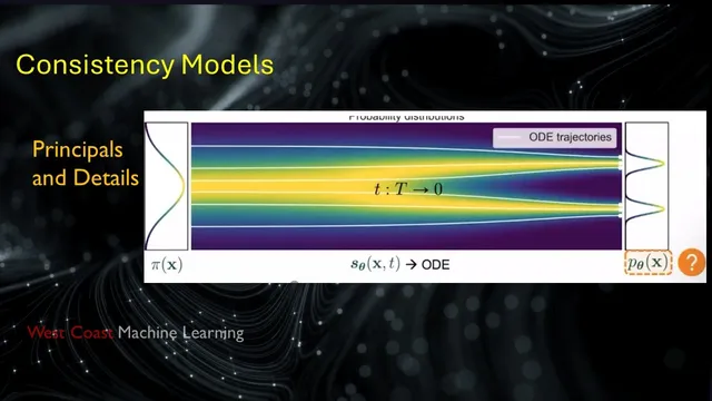
Consistency models aim to cut diffusion sampling time by replacing many denoising steps with a learned, one-step (or few-step) mapping from a noisy sample back to the data. The core idea rests on a mathematical link between diffusion’s stochastic differential equation (SDE) and a deterministic probability-flow ordinary differential equation (ODE): both describe the same evolution of probability densities. Once that bridge is in place, it becomes possible to train a neural network to “jump” along the ODE trajectory—taking an input at an intermediate noise level and producing the corresponding clean sample—without repeatedly evaluating the score model at many time steps.

The discussion begins with diffusion’s standard forward process: start from clean data, inject noise gradually until the distribution approaches a simple Gaussian prior, and then reverse the process to generate samples. In continuous time, the forward dynamics are modeled with an SDE whose drift and Brownian-motion terms progressively transform the data distribution into noise. The reverse dynamics are also an SDE, but its drift depends on the score function (the gradient of the log probability density). Training therefore learns a time-conditioned score network by minimizing a score-matching loss at randomly sampled time steps, then sampling uses an SDE solver to integrate the reverse process from Gaussian noise back toward the data manifold.

A key pivot comes from probability-flow ODEs. While the SDE produces stochastic trajectories, the ODE yields a deterministic path whose induced probability density matches the SDE’s at every time. This one-to-one correspondence between the SDE’s distribution evolution and the ODE’s deterministic flow enables a different training target: instead of repeatedly solving the reverse SDE, learn a function that maps directly from an intermediate noisy state to the clean state associated with that point on the ODE trajectory. In the simplest case, the learned function f_θ takes x_t (a noisy sample at time t) and outputs x_0 in a single step, provided the time conditioning is correct.

Consistency models formalize this with two constraints. First is a boundary condition near the smallest time ε: when the input is extremely close to the data, the model should output the same clean sample rather than collapsing to a constant. Second is a self-consistency constraint: for two time stamps t and t′ along the same probability-flow trajectory, applying f_θ at the correct time should return the same x_0. Architecturally, skip connections are used to enforce the ε behavior, and training samples pairs of adjacent (or near-adjacent) points along trajectories.

Training is presented in two main flavors. The more common approach distills from a pre-trained diffusion model: use an ODE solver to generate trajectory points, then train f_θ so that predictions from consecutive times agree on x_0. To stabilize learning and reduce gradient variance, a target network updated via exponential moving average (EMA) is used. The second approach trains a standalone consistency model without relying on a pre-trained diffusion model or an ODE solver, but it tends to be less effective because the added noise is not aligned with the specific trajectory structure.

Finally, sampling can be done in one step for speed, but quality improves with multi-step consistency sampling: repeatedly add analytically computed noise to the current estimate at later time steps and re-apply f_θ. The result is a practical tradeoff—fast generation with a small number of model evaluations—while retaining diffusion’s ability to model complex image distributions. The discussion also notes that consistency ideas extend beyond pixel space into latent-space variants (e.g., latent consistency models) and are already used in real-time image generation demos, though quality depends on the specific variant and training setup.