Convolutions | Why X+Y in probability is a beautiful mess

TL;DR

Convolution is the mechanism that converts two independent distributions into the distribution of their sum.

Briefing Cornell Notes

Briefing

Adding two independent random variables isn’t just a matter of “adding their means”—it reshapes their entire probability distribution through a specific operation called convolution. The core insight is that the distribution of the sum is built by combining the two underlying distributions in a structured way: for every possible target sum s, you multiply matching pieces of probability density (or probability mass in the discrete case) and then aggregate those products. That mechanism explains why normal distributions keep reappearing, and it sets up the central limit theorem as a repeated “smoothing” process.

The lesson begins with a discrete warm-up: two weighted dice are rolled independently, and the probability of each possible sum is computed precisely. One visualization treats the joint outcomes as a 6×6 multiplication table of probabilities (products of the blue die’s probabilities and the red die’s probabilities). To get the probability of a particular sum, all entries that lie on the diagonal corresponding to that sum are added together—so the sum distribution is like collapsing the table along diagonal slices. A second visualization flips one die’s distribution and slides it across the other; at each shift, the probability of a given sum becomes a dot-product-like accumulation of aligned probability pairs. Both views describe the same operation, just from different angles.

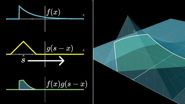
From there, the discussion generalizes to continuous random variables, where “probability” becomes “probability density” and sums become integrals. If f(x) and g(y) are density functions for two independent variables X and Y, then the density of S = X + Y is obtained by integrating the product f(x)·g(s − x) over all real x. An interactive geometric interpretation makes the formula feel less like an abstract definition: g(s − x) is a horizontally flipped and shifted version of g, and the convolution at input s equals the area under the product curve of f(x) and g(s − x). A concrete example uses two uniform distributions on [−1/2, 1/2], producing a triangular (wedge) distribution for the sum; extending to three uniforms is done by convolving the wedge with another top-hat, yielding a smoother, more bell-like shape.

Repeatedly convolving (equivalently, repeatedly adding independent copies) turns these increasingly smooth shapes into something arbitrarily close to a normal distribution after appropriate rescaling. This is the central limit theorem in functional form: convolution acts like a moving average that progressively suppresses irregularities, making the normal distribution an attractive fixed point. The “why normal?” question is then tied back to geometry using a final visualization: in the x–y plane, independence makes the joint density proportional to f(x)g(y). Restricting to the line x + y = s corresponds to diagonal slices of that surface, and integrating along those slices yields the convolution (up to a constant factor). The diagonal-slice view also makes convolution’s symmetry clear: f * g matches g * f, with only a scaling difference from how slice lengths map in the plane.

The payoff is practical: the diagonal-slice picture is positioned as a powerful route to compute the sum of two normal distributions, with the full proof deferred to the next installment.

Cornell Notes

Convolution is the operation that turns two independent probability distributions into the distribution of their sum. In the discrete dice example, probabilities form a grid of products, and the probability of a given total comes from adding the entries along the diagonal where x + y equals that total. In the continuous case, the same idea becomes an integral: the density of S = X + Y at value s is ∫ f(x) g(s − x) dx, interpreted geometrically as the area under the product of f(x) and a shifted/flipped version of g. Repeating this process (adding more independent copies) smooths shapes toward a bell curve, which is the central limit theorem. The diagonal-slice geometry also clarifies why convolution is symmetric and why normal distributions dominate.

Why does the probability of a specific sum come from “diagonal slices” in the dice example?

For two independent dice, each joint outcome (blue value x, red value y) has probability p_X(x)·p_Y(y). All outcomes that share the same sum s satisfy x + y = s, which forms a diagonal in the 6×6 grid of (x, y) pairs. Summing probabilities for all pairs on that diagonal adds exactly the probability that X + Y equals s.

How does the discrete “add along diagonals” idea translate to continuous convolution?

In continuous settings, probability mass becomes probability density, and “adding over discrete values” becomes integrating. The density of S = X + Y at s is computed by integrating over all x: f(x)·g(s − x). The term g(s − x) enforces the constraint that y must equal s − x so that x + y = s.

What does shifting and flipping g(s − x) mean geometrically?

Replacing y with s − x effectively flips g horizontally (because of the minus sign) and then shifts it by s. As s changes, the overlap between f(x) and g(s − x) changes; the convolution value is the area under their product curve for that particular shift.

Why does adding more uniform variables produce a smoother shape that trends toward a bell curve?

A uniform “top hat” convolved with another top hat yields a wedge (triangular) distribution because overlap grows linearly and then shrinks linearly. Convolving that wedge again with a top hat corresponds to a moving-average-like smoothing: the result tapers more smoothly. Repeating this smoothing many times, with rescaling, drives the shape toward a normal distribution.

How does the x–y surface and diagonal slice visualization explain convolution and its symmetry?

Independence makes the joint density proportional to f(x)g(y), forming a surface over the x–y plane. Fixing S = x + y = s restricts attention to the diagonal line x + y = s. Integrating (slicing) along that diagonal produces the convolution value. This view makes symmetry intuitive: swapping f and g corresponds to the same diagonal-slice construction, differing only by a constant scaling factor (involving √2) from how slice lengths map.

Review Questions

In the continuous convolution formula ∫ f(x) g(s − x) dx, what role does the term (s − x) play in enforcing the constraint x + y = s?
Using the diagonal-slice idea, what changes when you increase s: the set of (x, y) pairs considered, or the integrand’s shape, or both?
Why does repeated convolution require rescaling to match the standard central limit theorem statement?

Key Points

1
Convolution is the mechanism that converts two independent distributions into the distribution of their sum.
2
In the discrete case, the sum distribution is obtained by multiplying independent probabilities for each (x, y) pair and then adding along diagonals where x + y is constant.
3
In the continuous case, the same logic becomes an integral: the density at s is ∫ f(x) g(s − x) dx.
4
Geometrically, convolution at s equals the area under the product of f(x) and a flipped-and-shifted version of g.
5
Convolving uniform distributions repeatedly yields progressively smoother shapes, matching the intuition behind the central limit theorem.
6
The diagonal-slice visualization links convolution to integrating joint density f(x)g(y) along lines x + y = s, making symmetry (f * g = g * f) clear up to a scaling factor.
7
The normal distribution emerges as an attractive fixed point under repeated convolution after appropriate rescaling.

Highlights

The probability of a sum s is built by multiplying matching probability pieces (x with y = s − x) and then aggregating them—diagonals in the discrete grid, slices/areas in the continuous plane.

Convolution can be read as “moving overlap”: flip g, slide it across f, and the convolution value is the area under their product for each shift.

Uniform + Uniform gives a wedge-shaped distribution; adding more uniforms repeatedly smooths the shape toward a bell curve.

Independence turns the joint density into a product surface f(x)g(y), and conditioning on x + y = s corresponds to diagonal slices whose areas yield the convolution (with a √2 scaling detail).