Creating A Reinforcement Learning (RL) Environment - Reinforcement Learning p.4

A simple grid-world built from scratch lets a Q-learning agent learn to reach a “food” blob while avoiding an “enemy” blob—despite having no explicit knowledge of walls or boundaries. The environment uses relative positions (player-to-food and player-to-enemy deltas) as the observation, a small discrete action set for movement, and a tabular Q-table updated with standard Q-learning. The striking result: the agent can still succeed at high rates, often by using the walls as an accidental navigation aid, even though it never “learns” wall geometry directly.

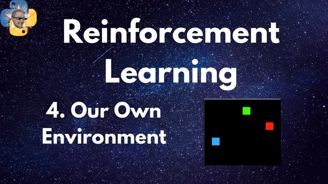
The setup starts with a 10×10 grid. Three blobs are initialized at random coordinates: the player (blue), the food (green), and the enemy (red). In the early training mode, only the player moves; food and enemy remain stationary. The reward structure is tuned to push behavior: hitting the enemy ends the episode with a large negative penalty (enemy penalty set to 300), reaching the food ends the episode with a positive reward (food reward set to 25), and every other move incurs a small negative move penalty (−1). Exploration is controlled by epsilon-greedy policy: epsilon begins at 0.9 and decays over 25,000 episodes.

Instead of feeding absolute coordinates, the observation is built from relative geometry. A custom blob class supports operator overloading so the code can compute (player − food) and (player − enemy), producing a tuple of coordinate deltas. That tuple becomes the key into a dictionary-based Q-table. Because there are two relative position pairs, the Q-table effectively stores Q-values for every combination of those deltas, with four discrete actions corresponding to diagonal moves (choice 0–3). The move method also clamps positions to the grid edges: if the player attempts to step outside the 0–9 range, it gets snapped back to the boundary.

Training iterates over episodes and steps (200 steps per episode). For each step, the agent chooses either a random action (with probability epsilon) or the action with the highest Q-value for the current observation. After moving, it recomputes the new observation, calculates the reward (food, enemy, or move penalty), and updates the Q-table using the Q-learning update rule with a learning rate of 0.1 and a discount factor of 0.95. When food or enemy is reached, the episode terminates; otherwise it continues.

Visualization is done with OpenCV: the grid is rendered as an RGB image, scaled up for display, and refreshed each step. After training, the learned Q-table is saved via pickle and can be reloaded for evaluation with epsilon set to 0 (pure exploitation). The agent’s behavior becomes visibly competent: it zigzags toward the food and, in many cases, “bounces” off walls to reach otherwise hard-to-access positions.

Scaling experiments highlight a practical cost of tabular methods. Increasing the grid from 10×10 to 20×20 causes the Q-table size to balloon—from roughly 15 MB to about 250 MB. Yet the agent still learns in the larger environment, including when movement is enabled for both food and enemy, sometimes handling more complex avoidance and pursuit dynamics. The overall takeaway is that even a constrained, wall-agnostic tabular setup can produce surprisingly effective navigation—while also demonstrating why state/action explosion quickly makes Q-tables unwieldy.