Data Distribution/Normality in PLS SEM using SmartPLS

PLS-SEM work in SmartPLS often raises a practical question: should researchers test whether survey responses are normally distributed? The core takeaway is that PLS-SEM doesn’t rely on strict normality assumptions the way covariance-based SEM does, but normality still matters because extreme non-normality can distort results. Since survey data are recorded across fixed response categories (e.g., 1–7 agree/disagree scales), researchers can summarize how responses cluster across categories using frequency tables, bar charts, or histograms—then assess whether the overall pattern resembles a bell-shaped normal curve.

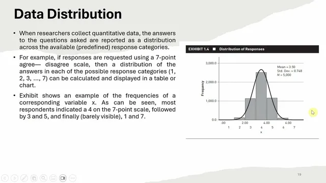
In the transcript’s example, most respondents select the middle categories (around 4 on a 7-point scale), with fewer responses at the extremes (1 and 7). That “bell-shaped” pattern is the hallmark of a normal distribution: values concentrate near the mean and thin out toward both tails. Real data, however, can deviate from normality in predictable ways, such as becoming skewed (asymmetry) or having heavy/light tails (captured by kurtosis). Rather than relying on a single visual check, the recommended approach is to quantify deviation from normality.

For PLS-SEM, the transcript notes that formal normality tests like the Shapiro–Wilk test or other goodness-of-fit tests (e.g., “cgov smof”) can be applied, but in practice many researchers focus on two distribution diagnostics: skewness and kurtosis. Skewness indicates whether the distribution leans left or right; kurtosis reflects how peaked or flat the distribution is and how heavy the tails are. Common rule-of-thumb thresholds are mentioned: skewness is typically expected to fall within about ±2, while kurtosis is often considered acceptable up to around 5 (with some references allowing values up to 10). The transcript also points to established SEM methodology references (including guidance attributed to Hair, Black, Babin, and Anderson, and a note about Joel Kier’s discussion of kurtosis ranges).

The workflow in SmartPLS is straightforward. After loading the dataset, researchers can inspect skewness and kurtosis values directly in the software’s output (the transcript points to the “skewness and kosis” section). If both metrics sit comfortably within the cited ranges—no extreme violations—analysis can proceed without concern for normality-driven distortions. If values fall outside those bounds, the transcript’s logic implies the need for caution and potentially further steps, because the distribution may be materially non-normal even if PLS-SEM itself is more forgiving than covariance-based SEM.

Overall, the message is balanced: PLS-SEM may not require normality by assumption, but distribution checks remain a safeguard against outlier-heavy or strongly asymmetric survey patterns that could undermine inference.