First Basic Model using GSCA in #SmartPLS
Based on Research With Fawad's video on YouTube. If you like this content, support the original creators by watching, liking and subscribing to their content.
GSCA in SmartPLS estimates path relationships between observed variables and components while producing dedicated model fit statistics.
Briefing
Generalized Structured Component Analysis (GSCA) in SmartPLS is presented as a new way to run structural equation models that estimates path relationships between observed variables and components. The core practical takeaway is that GSCA lets researchers keep the same modeling workflow—dragging constructs, connecting paths, and calculating results—while adding a clear set of model fit outputs to judge how well the specification accounts for the observed data.
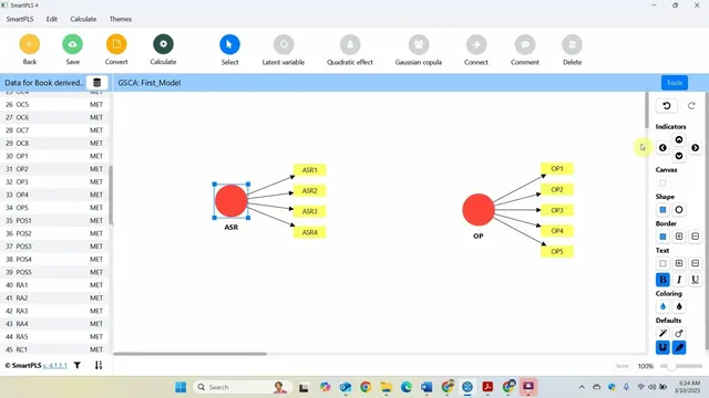
In the session, a GSCA model is created using an existing project and data set. The model type is switched to GSCA, a first model is saved, and the researcher specifies the structural relationship of interest: the impact of “assurance” on “organizational performance.” Once the path is connected and the model is calculated, the output includes familiar measurement and structural elements. Outer loadings are reported for the measurement side, and the results are described as matching what would be obtained under earlier approaches—highlighting that the technique changes, not the basic interpretation of loadings and relationships. Reliability and validity checks also appear, including composite reliability (not shown in the immediate view but indicated as available), along with discriminant validity presented in graphical form.
The main difference emphasized comes with model fit assessment. GSCA provides multiple fit statistics, including SRMR and fit indices intended to quantify how closely the estimated model reproduces the observed data. The guidance given is straightforward: SRMR values below 0.08 (closer to zero) indicate better fit, while fit indices closer to 1 are better. These fit measures are described as adjusted for free parameters, and local fit indices are also available for later discussion.
To interpret the fit numerically, the session points to a variance-explained framing. Fit values are treated as ranging from 0 to 1 and interpreted as the variance accounted for by the model specification. The example results include a fit around 0.646, described as explaining roughly 64.6% of the variance, and an additional output indicating about 50% of the variance of all variables is explained by the model. Together, these are used to label the model fit as “reasonable.”
Finally, hypothesis testing is carried out through bootstrapping. The session recommends running bootstrapping with 5,000 resamples, using bias-corrected and a one-tailed test setting. The resulting path coefficients show statistical significance, leading to the conclusion that assurance has a significant and positive impact on organizational performance. The walkthrough ends by noting that the same GSCA approach can be extended later into more complex models.
Cornell Notes
GSCA in SmartPLS provides an alternative structural equation modeling approach that estimates relationships between observed variables and components while also producing model fit statistics. In a basic example, assurance is linked to organizational performance, and the workflow mirrors earlier SmartPLS modeling: connect paths, calculate, and review outer loadings plus reliability and validity outputs. The session highlights GSCA’s fit reporting—especially SRMR (values < 0.08 are better) and fit indices closer to 1—along with variance-explained interpretations (e.g., about 64.6% variance accounted for). Hypotheses are tested using bootstrapping with 5,000 resamples, bias-corrected settings, and a one-tailed test, yielding a significant positive path from assurance to organizational performance.
What does GSCA add to a SmartPLS workflow compared with earlier SEM approaches?
How is the measurement side checked after running a basic GSCA model?
How should SRMR and fit indices be interpreted in this GSCA example?
What variance-explained interpretation is used for GSCA fit values?
How are hypotheses tested after estimating a GSCA model in SmartPLS?
Review Questions
- In a GSCA model, which fit statistic is used here to judge absolute fit, and what threshold is given for it?
- How does the session interpret fit values numerically in terms of variance explained?
- What bootstrapping settings are used for hypothesis testing, and how do they affect the path significance check?
Key Points
- 1
GSCA in SmartPLS estimates path relationships between observed variables and components while producing dedicated model fit statistics.
- 2
A basic GSCA workflow can reuse an existing SmartPLS project: set model type to GSCA, save, connect paths, and calculate.
- 3
Outer loadings and reliability/validity outputs (including discriminant validity) are reviewed after calculation, similar to earlier SEM approaches.
- 4
Model fit is assessed using SRMR (values < 0.08 are treated as good) and fit indices (closer to 1 is treated as better).
- 5
Fit indices are interpreted as variance accounted for by the model specification, enabling percentage-style statements about explained variance.
- 6
Hypothesis testing is performed with bootstrapping (5,000 resamples, bias-corrected, one-tailed), and significant path coefficients support directional claims.