Generative Model That Won 2024 Nobel Prize
Based on Artem Kirsanov's video on YouTube. If you like this content, support the original creators by watching, liking and subscribing to their content.
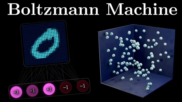
Boltzmann machines replace deterministic energy descent with stochastic sampling using probabilities proportional to exp(−E/T), normalized by the partition function Z.
Briefing
Boltzmann machines turned neural networks from rigid “energy minimizers” into probabilistic generators by injecting randomness into both inference and learning. Instead of always settling into the single lowest-energy configuration (as in Hopfield-style associative memory), Boltzmann machines sample states according to the Boltzmann distribution—making it possible to escape local minima, represent uncertainty, and generate new outputs that were never explicitly stored.
The foundation starts with Hopfield networks, which assign an energy to every possible neuron state and then iteratively descend the energy landscape until the system falls into the nearest “well,” effectively completing a stored pattern from partial input. That mechanism is excellent for recall, but it mostly reproduces what was learned; it doesn’t naturally model the probability structure behind the data. Boltzmann machines address that gap with two key upgrades: stochasticity and hidden units.
Stochasticity comes from physics. Ludwig Boltzmann’s work on gas particles links the probability of a state to its energy via an exponential rule: lower-energy states are exponentially more likely, with temperature controlling how sharply probability concentrates. The missing piece is normalization: absolute probabilities require the partition function Z, which sums exponentiated negative energies across all states. Once that probability rule is in hand, a Hopfield neuron update can be turned into a probabilistic one. Holding the rest of the network fixed, the chance that a particular neuron turns “on” becomes a sigmoid function of its weighted input. A random draw then decides whether the neuron switches, with high “temperature” producing more randomness and low “temperature” recovering near-deterministic Hopfield behavior.
Learning changes just as dramatically. Hopfield learning aims to lower energy for desired patterns. Boltzmann machines instead maximize the likelihood that the model assigns high probability to training data. That objective produces the contrastive Hebbian learning rule: a “positive phase” where visible units are clamped to real training examples and weights are updated using correlations observed under those constraints, and a “negative phase” where the network runs freely to sample its own equilibrium states. Weight updates strengthen correlations that appear with data but weaken those that appear when the model hallucinates—effectively shaping an energy landscape where data patterns become deep wells while unrealistic configurations are pushed upward.
Hidden units complete the story. Visible units correspond to observed inputs, while hidden units capture latent structure and higher-order correlations that aren’t directly encoded in the visible layer. During training, hidden units are not labeled; they evolve during the positive and negative phases, and the contrastive learning updates adjust weights connected to them so the model learns useful internal representations.
A practical variant, the restricted Boltzmann machine (RBM), forbids connections among visible-visible and hidden-hidden units, enabling parallel updates and faster training/inference while retaining much of the expressive power. Although modern generative AI often relies on back-propagation-trained multi-layer networks, the core principles Boltzmann machines introduced—probabilistic modeling of uncertainty and learning latent features—still underpin how today’s systems think about generation.
Cornell Notes
Boltzmann machines extend Hopfield networks by turning deterministic energy minimization into probabilistic sampling. Neurons update stochastically using probabilities derived from the Boltzmann distribution, where state probability is proportional to exp(−E/T) and normalized by the partition function Z. Learning then shifts from storing patterns to maximizing the likelihood of training data, producing the contrastive Hebbian rule with a positive phase (data clamped) and a negative phase (model samples freely). Hidden units let the model learn latent features and higher-order correlations without direct supervision. Restricted Boltzmann machines (RBMs) simplify connectivity to allow parallel updates, improving computational efficiency.
How does a Hopfield network recall stored patterns, and why does that limit creativity?
What does the Boltzmann distribution add to neural-network updates?
Why does temperature matter, and what happens in the extremes?
What is the contrastive learning objective, and how do the positive and negative phases differ?
How do hidden units enable Boltzmann machines to learn abstract structure?
Review Questions
- What role does the partition function Z play in converting relative energy-based probabilities into valid probability distributions?
- Describe how the positive and negative phases in contrastive Hebbian learning lead to different correlation measurements.
- Why does adding hidden units change what Boltzmann machines can represent compared with visible-only Hopfield-style networks?
Key Points
- 1
Boltzmann machines replace deterministic energy descent with stochastic sampling using probabilities proportional to exp(−E/T), normalized by the partition function Z.
- 2
A neuron’s on/off update probability becomes a sigmoid function of its weighted input, with random draws deciding the next state.
- 3
Learning shifts from storing patterns to maximizing the likelihood of training data, producing the contrastive Hebbian learning rule.
- 4
Contrastive learning uses a positive phase (data clamped) and a negative phase (free-running equilibrium) to strengthen data-consistent correlations and weaken model-generated ones.
- 5
Hidden units provide latent representations that capture abstract features and higher-order correlations without direct supervision.
- 6
Restricted Boltzmann machines (RBMs) restrict connectivity to enable parallel updates, making training and inference more efficient.
- 7
Temperature controls the trade-off between exploration (high T) and near-deterministic settling (low T), helping the model escape local minima.