How I make science animations

Science animations are built from a deliberately mixed toolkit: Python (for mathematically generated visuals), Blender (for true 3D), and Adobe After Effects (for composition, timing, and the final polish). The core workflow hinges on a practical rule—no single tool produces every piece cleanly—so the production pipeline assigns tasks to whichever software handles them best, then stitches the results together with tight synchronization.

After Effects is the “workhorse” for most simple animation and for assembling outputs from other programs into a final render. It’s favored because it hits a balance between capability and usability for tasks like styling text, animating elements onto screen, adding motion (wiggles, hue shifts), and transitioning scenes. More specialized effects—realistic explosions, keying, advanced color correction, 3D tracking—are left to dedicated tools when needed.

Python becomes essential when the animation can’t be done by hand or by After Effects scripting alone. After Effects’ JavaScript API is described as limited for complex, programmatic visualization tasks such as generating large numbers of connected elements that obey mathematical rules. Python’s strength is numerical control—variables, loops, recursion—and the ability to generate frames from math directly. Two Python libraries dominate this stage: Manim (originally developed by Grant Sanderson and now community-maintained) for earlier mathematical animation work, and matplotlib for more flexible, frame-by-frame control. Matplotlib is used for animations of plots being drawn and for visualizing complex systems (including examples like an Ising model and artificial neural networks). Manim still earns a place for graph animations thanks to its out-of-the-box graph-theory support.

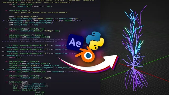
Blender is the go-to for 3D work because After Effects and Python are described as limited for full three-dimensional scenes. Blender’s Python API also enables programmatic 3D visualization, which matters for neuron-like objects, maze-running mice, and surface plots.

Around this backbone sits a supporting cast from Adobe: Illustrator for vector assets and diagrams that update cleanly inside After Effects; Photoshop for thumbnails and raster touch-ups like subject cutouts and minor color work; Premiere Pro for classic editing tasks like trimming, sequencing, and audio integration; and Adobe Audition for audio cleanup and enhancement (noise reduction, removing plosives, and reducing unwanted mouth sounds).

A detailed example shows how matplotlib and After Effects work together. A rotating arrow produces a sinusoid with time-varying frequency; matplotlib generates the wave and its frequency-related visuals as pre-rendered videos with thousands of frames. After Effects then handles layout, text, and synchronization to voice-over using time remapping. Black backgrounds from matplotlib are converted into transparency via blending modes (notably “Screen”), enabling layers to be arranged without obstruction. Gradient fills are created in After Effects by using gradient ramps and masking techniques to recolor a white fill only where needed. The “squishing” and morphing steps rely on seamless stitching: the final frame of one matplotlib render matches the initial frame of the next, so After Effects can transition between them while time remapping controls pacing.

The same pipeline logic extends to more ambitious projects: biophysically accurate neuron voltage propagation built via a Blender add-on (“Blender Spike”) that imports simulation results into Blender; probability-distribution slicing created by generating height maps with matplotlib and displacing Blender grids, then using node-based shader mixing to reveal thin cut lines; importing brain atlas meshes via Brain Globe API and a helper add-on (“BlenderBrain”); and a branching-model information transmission animation where network states are simulated in Python, then smoothed using convolution (SciPy) to avoid choppy frame-by-frame switching. Even rearranging neuron layouts is handled by combining simulation data with Manim graph objects and coordinated animations.

Across all these examples, the takeaway is operational: generate the math-driven building blocks programmatically, over-render for flexible timing, and let After Effects orchestrate composition and synchronization—often with time remapping as the key control lever.