How to Convert a Continuous Variable in to a Categorical Variable using SPSS?

TL;DR

Identify the observed minimum and maximum values of the continuous age variable before defining age-group intervals.

Briefing Cornell Notes

Briefing

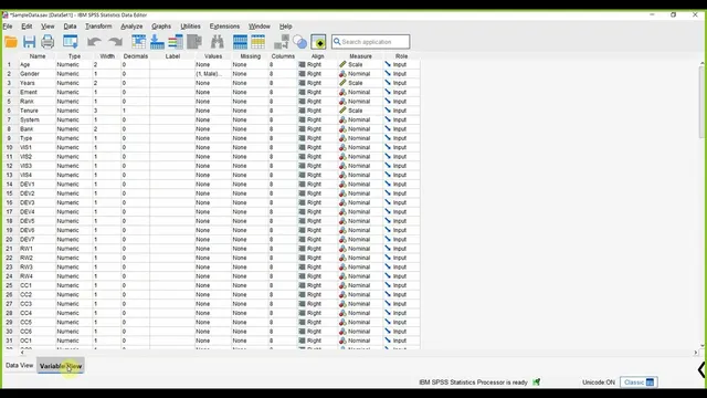
Turning a continuous age variable into clear “age group” categories in SPSS starts with defining the minimum and maximum values, then building recoding ranges that match the thesis table format. With ages running from 20 to 59, the categories can be set as 20–29, 30–39, 40–49, and 52–59 (each assigned a numeric code such as 1 through 4). In SPSS, this is done under Transform → Recode into Different Variables, where the original age variable is recoded into a new variable (for example, AG_gr). The recode uses the “Range” option so that each age interval maps to a specific code: 20–29 becomes 1, 30–39 becomes 2, 40–49 becomes 3, and 52–59 becomes 4.

Once the new categorical variable exists, the next step is choosing the right SPSS output so the results are thesis-ready. If descriptive statistics are run on the coded variable, the output may show a mean like 1.91—technically correct but not meaningful to readers because it’s expressed in category codes rather than age ranges. The more useful approach is Analyze → Descriptive Statistics → Frequencies using the new age-group variable. This produces a frequency table listing each code (1, 2, 3, 4) and the number of respondents in each group.

However, the frequency table still isn’t reader-friendly until the codes are labeled. SPSS can attach value labels to the categorical variable: go to the variable’s “Values” settings and define what each numeric code represents. For example, label 1 as “20 to 29,” 2 as “30 to 39,” 3 as “40 to 49,” and 4 as “52 to 59.” After applying these value labels, rerunning Frequencies yields a table where readers immediately see the age ranges alongside the respondent counts—exactly what’s needed for an APA-style thesis table showing age group, frequency, and percentage.

In short: define age-group ranges from the observed minimum and maximum, recode the continuous age into a new categorical variable using SPSS’s range-based recoding, then label the resulting codes so frequency outputs communicate the actual age intervals instead of abstract numbers.

Cornell Notes

A continuous age variable (20–59) can be converted into a categorical “age group” variable in SPSS by recoding it into defined ranges. The process uses Transform → Recode into Different Variables to create a new variable (e.g., AG_gr) and assigns numeric codes to each interval (1 for 20–29, 2 for 30–39, 3 for 40–49, 4 for 52–59). Running Frequencies on the coded variable gives counts per code, but the table becomes meaningful only after adding value labels that map each code to its age range. This produces thesis-ready output showing respondent frequencies by age group (and supports APA-style tables).

Why is it not enough to run Descriptives on the recoded age-group variable?

Descriptives on the coded variable reports statistics in terms of the numeric category codes (e.g., a mean of 1.91). That number doesn’t tell a reader what age range it corresponds to. Frequencies plus value labels communicates the actual intervals (like 20–29) alongside respondent counts, which is what thesis tables need.

What SPSS steps create a new categorical age-group variable from a continuous age variable?

Use Transform → Recode into Different Variables. Select the original age variable, specify a new variable name (such as AG_gr), then click Old and New Values. Choose Range and define the intervals (e.g., 20–29 → 1, 30–39 → 2, 40–49 → 3, 52–59 → 4). After confirming, SPSS creates the new categorical variable.

How do Frequencies and value labels work together to make results readable?

Frequencies produces a table with codes (1, 2, 3, 4) and the number of respondents in each category. To make the table understandable, assign value labels: open the variable’s Values settings and label each code with its age range (1 = 20 to 29, 2 = 30 to 39, 3 = 40 to 49, 4 = 52 to 59). After labeling, rerunning Frequencies shows age ranges instead of abstract codes.

What information should be determined before recoding age into categories?

Before recoding, identify the minimum and maximum values of the age variable. Those endpoints determine the overall span of the categories. In this example, ages run from 20 (minimum) to 59 (maximum), which guides the selection of age-group intervals.

What does the frequency table output represent after recoding?

After recoding and labeling, the frequency table lists each age group and the count of respondents in that group. For instance, one code corresponds to 20–29 with a specific respondent frequency, and the other codes correspond to the remaining age intervals (30–39, 40–49, 52–59).

Review Questions

What SPSS menu path converts a continuous variable into a categorical variable using recoding?
How would you interpret a mean value like 1.91 for a recoded age-group variable, and why is it less useful than a labeled frequency table?
What steps turn a frequency table with codes (1–4) into a thesis-ready table with age ranges?

Key Points

1
Identify the observed minimum and maximum values of the continuous age variable before defining age-group intervals.
2
Create a new categorical variable in SPSS using Transform → Recode into Different Variables.
3
Use the “Range” option in recoding so each age interval maps to a specific numeric code.
4
Run Analyze → Descriptive Statistics → Frequencies on the new categorical variable to get respondent counts per group.
5
Add value labels to map each numeric code to its corresponding age range so readers understand the categories.
6
Prefer labeled frequency output over Descriptives on coded categories, since coded means (e.g., 1.91) are not reader-friendly.

Highlights

Recoding age 20–59 into four labeled groups (20–29, 30–39, 40–49, 52–59) turns a continuous variable into thesis-ready categories.

Frequencies provides the counts per category, but value labels are required to replace codes (1–4) with real age ranges.

A mean like 1.91 from Descriptives on coded categories is mathematically valid yet not interpretable for readers without labels.

Topics

SPSS Recoding
Categorical Variables
Value Labels
Frequencies Tables
Age Grouping