Lecture 1: Deep Learning Fundamentals (Full Stack Deep Learning - Spring 2021)
Based on The Full Stack's video on YouTube. If you like this content, support the original creators by watching, liking and subscribing to their content.
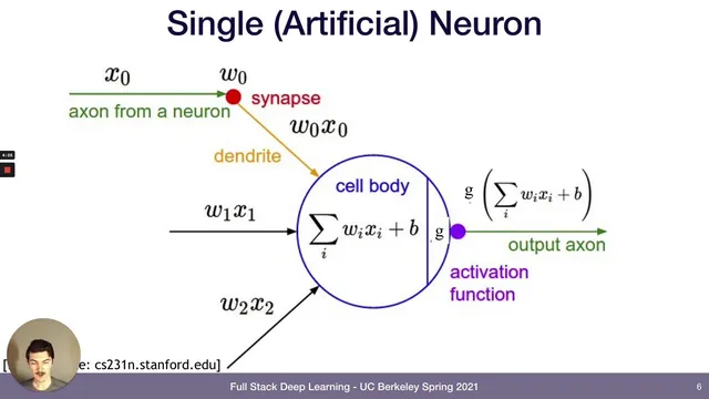
Neural networks are built by stacking perceptrons: weighted sums plus biases followed by nonlinear activations like ReLU.
Briefing
Deep learning fundamentals hinge on a simple but powerful idea: neural networks are flexible function approximators whose weights can be trained by minimizing a loss function using gradient-based optimization. That combination—universal approximation plus practical training via gradient descent and back propagation—explains why neural networks can tackle everything from image recognition to language modeling, and why modern compute (especially GPUs) made the approach scalable.
The lecture starts with the biological metaphor of neurons, then translates it into the perceptron: inputs are weighted (w) and shifted by a bias (b), summed, and passed through an activation function that decides whether the neuron “fires.” Classic activations like the sigmoid squash outputs into a 0–1 range, while hyperbolic tangent offers a similar smooth nonlinearity. The modern workhorse is the rectified linear unit (ReLU), defined as max(0, x), which outputs zero for negative inputs and passes positive values through. ReLU’s gradient is simple (1 when x>0, otherwise 0), and its adoption is credited as a key ingredient in the deep learning revival around 2013.
Neural networks become “networks” by stacking perceptrons into layers: an input layer, one or more hidden layers, and an output layer. Each layer’s weights and biases determine how the model transforms inputs into predictions. Theoretical results support the intuition that sufficiently wide two-layer networks (one hidden layer) can approximate essentially any function—this is the universal approximation theorem. The intuition offered is that many hidden units can act like a collection of “basis” components that combine to reproduce complex shapes, reminiscent of how Fourier-style representations can model complicated signals.
From there, the lecture maps neural networks onto major machine learning problem types. Supervised learning trains on labeled pairs (x, y), such as images mapped to categories (cat/not cat) or audio mapped to spoken content. Unsupervised learning uses unlabeled data (x only) to discover structure—examples include next-character prediction for language modeling, learning word relationships via vector representations, and learning compact image representations through compression and reconstruction. Reinforcement learning trains an agent to choose actions in an environment, receiving feedback as rewards; the state changes after each action, and the goal is to learn strategies that maximize long-term outcomes.
Training is framed as empirical risk minimization: choose model parameters to minimize a loss function. For regression, squared error is a common loss; for classification, cross entropy loss is typical because outputs correspond to discrete categories. Optimization proceeds with gradient descent: update each parameter by moving opposite the gradient of the loss, scaled by a learning rate (α). Because full-dataset updates are expensive, the lecture emphasizes stochastic and mini-batch variants that trade noisier updates for faster progress. Back propagation then provides an efficient way to compute gradients through layered computations using the chain rule, typically handled automatically by tools like PyTorch or TensorFlow.
Finally, architectural choices and compute infrastructure matter. Convolutional networks encode locality for vision, recurrent networks capture sequence structure, and techniques like skip connections help gradient flow in deeper models. The deep learning boom is also tied to better GPU support: Nvidia CUDA enabled GPUs—originally built for graphics—to accelerate the matrix multiplications that dominate neural network workloads, making large-scale training practical.
Cornell Notes
Neural networks model a function y = f(x) by stacking perceptrons (weighted sums plus biases) and passing results through activation functions such as sigmoid, tanh, and especially ReLU. Theory supports their flexibility: two-layer networks with enough hidden units can approximate essentially any function (universal approximation). Training is posed as minimizing a loss function (squared error for regression; cross entropy for classification) using gradient descent variants like stochastic or mini-batch gradient descent. Back propagation efficiently computes gradients through the network via the chain rule, usually via automatic differentiation in frameworks such as PyTorch or TensorFlow. Practical performance depends on architecture (e.g., convolutional nets for vision, recurrent nets for sequences, skip connections) and on GPU acceleration through Nvidia CUDA, which speeds up the matrix multiplications at the core of deep learning.
How does a perceptron turn inputs into an output, and why do activation functions matter?
What does “universal approximation” mean in practical terms?
How do supervised, unsupervised, and reinforcement learning differ by what data and feedback they use?
What is a loss function, and how does minimizing it lead to training?
Why do gradient descent variants like SGD exist, and what role does back propagation play?
How do architecture choices and GPU compute (CUDA) connect to real-world deep learning performance?
Review Questions
- What changes in the loss function when moving from regression to classification, and why?
- Describe the training loop: how do learning rate, gradients, and parameter updates work together?
- Give one example each of supervised, unsupervised, and reinforcement learning, and specify what the model receives as input and feedback.
Key Points
- 1
Neural networks are built by stacking perceptrons: weighted sums plus biases followed by nonlinear activations like ReLU.
- 2
Universal approximation theory supports the idea that sufficiently large two-layer networks can approximate essentially any function.
- 3
Supervised learning uses labeled pairs (x, y), unsupervised learning uses unlabeled inputs x to discover structure, and reinforcement learning uses rewards from an environment after actions.
- 4
Training is empirical risk minimization: choose weights and biases to minimize a loss function (squared error for regression; cross entropy for classification).
- 5
Gradient descent updates parameters by subtracting the learning rate times the gradient of the loss; mini-batch and stochastic variants reduce compute per step.
- 6
Back propagation computes gradients efficiently through layered networks using the chain rule, typically via automatic differentiation in PyTorch or TensorFlow.
- 7
Deep learning performance depends on architecture (convolutions for vision, recurrence for sequences, skip connections for deeper models) and GPU acceleration via Nvidia CUDA for fast matrix multiplications.