Multivariable Calculus 25 | Implicit Function Theorem
Based on The Bright Side of Mathematics's video on YouTube. If you like this content, support the original creators by watching, liking and subscribing to their content.
Assume F:U→R^M is C^1 on an open set U⊂R^{K+M} and that F(x0,y0)=0 at a chosen point.
Briefing
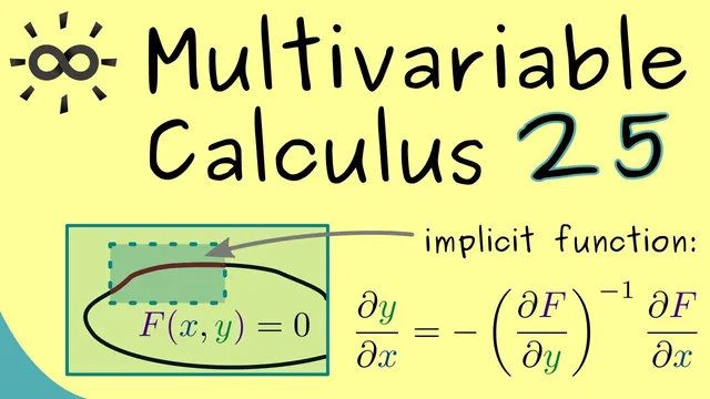
The implicit function theorem turns “messy” equations into locally well-behaved functions—provided the right Jacobian block is invertible. In practical terms, if a system of M equations in N=K+M variables can be written as F(x,y)=0 with x∈R^K and y∈R^M, then near a solution point (x0,y0) the solutions form a local graph y=G(x). That matters because it converts a contour-like set (which can fold and fail to be a function globally) into something that behaves like a function in a neighborhood, enabling differentiation and computation.
The setup starts with an open domain U⊂R^N and a C^1 map F:U→R^M. Choose a point u0=(x0,y0) in U such that F(u0)=0 (the zero vector in R^M). Writing the Jacobian of F at u0 in block form separates derivatives with respect to the first K variables (x) from derivatives with respect to the last M variables (y). Concretely, the Jacobian splits into an M×K matrix DF/DX and an M×M matrix DF/DY, where DF/DY collects all partial derivatives of the vector-valued F with respect to the y-variables.
The key condition is that the M×M matrix DF/DY evaluated at u0 is invertible—equivalently, its determinant is nonzero. Geometrically, this rules out “bad” points where the solution set would not locally look like a graph over the x-coordinates (for instance, a contour line that turns back on itself). Once this invertibility holds, the theorem guarantees the existence of open neighborhoods V1⊂R^K around x0 and V2⊂R^M around y0, along with a C^1 function G:V1→V2 such that every nearby solution satisfies y=G(x). In other words, within V1×V2, the set of points (x,y) with F(x,y)=0 is exactly the graph of G.
Beyond existence, the theorem provides a concrete differentiation formula. For x near x0, the Jacobian of G is given by
DG/DX = −(DF/DY)^{-1} · (DF/DX),
with both Jacobian blocks evaluated at the corresponding point (x,G(x))—in particular at u0 when x=x0. This relationship is the computational payoff: even when G’s explicit formula is unknown, its derivative can be computed from the derivatives of F. The result is a local justification for treating implicit equations as defining functions, which underpins later examples and applications in multivariable calculus.
Cornell Notes
The implicit function theorem addresses systems F(x,y)=0 where x∈R^K, y∈R^M, and F:U→R^M is C^1 on an open set U⊂R^{K+M}. If a point (x0,y0) satisfies F(x0,y0)=0 and the M×M Jacobian block DF/DY at (x0,y0) is invertible (determinant nonzero), then nearby solutions form a local graph y=G(x) for some C^1 function G defined on a neighborhood of x0. The theorem also gives a derivative formula: DG/DX = −(DF/DY)^{-1}(DF/DX), evaluated at (x,G(x)). This matters because it converts a contour-like solution set into a differentiable function locally, enabling calculations without solving the system explicitly.
What does it mean for the solution set of F(x,y)=0 to become a “local graph” y=G(x)?
Why is invertibility of DF/DY the decisive condition?
How does the theorem generalize the single-variable implicit function idea to multiple equations?
What is the block structure of the Jacobian in this setting?
How is the derivative of the implicit function G computed without an explicit formula for G?
Review Questions
- In the theorem’s notation, what are the dimensions of DF/DX and DF/DY when x∈R^K and y∈R^M?
- What geometric failure does the invertibility of DF/DY prevent, and how does that relate to representing the solution set as y=G(x)?
- Using the derivative formula, how would you compute DG/DX at x0 if you know the Jacobian blocks of F at (x0,y0)?
Key Points
- 1
Assume F:U→R^M is C^1 on an open set U⊂R^{K+M} and that F(x0,y0)=0 at a chosen point.
- 2
Split variables as x∈R^K and y∈R^M, and form the Jacobian blocks DF/DX (M×K) and DF/DY (M×M).
- 3
Require DF/DY evaluated at (x0,y0) to be invertible (determinant nonzero) to ensure local solvability for y in terms of x.
- 4
Under that condition, there exist neighborhoods V1⊂R^K and V2⊂R^M and a C^1 function G:V1→V2 such that all nearby solutions satisfy y=G(x).
- 5
Within V1×V2, the set { (x,y) : F(x,y)=0 } equals the graph of G, so no other contour pieces appear in that rectangle.
- 6
The Jacobian of G is computable via DG/DX = −(DF/DY)^{-1}(DF/DX), evaluated at (x,G(x)).